We have laid out the need for statistical analysis of paleomagnetic data in the preceding chapters. For instance, we require a method for determining a mean direction from a set of observations. Such a method should provide some measure of uncertainty of the mean direction. Additionally, we need methods for assessing the significance of field tests of paleomagnetic stability. In this chapter, we introduce basic statistical methods for analysis of directional data. It is sometimes said that statistical analyses are used by scientists in the same manner that a drunk uses a light pole: more for support than for illumination. Although this might be true, statistical analysis is fundamental to any paleomagnetic investigation. An appreciation of the basic statistical methods is required to understand paleomagnetism.
Most of the statistical methods used in paleomagnetism have direct analogies to “planar” statistics. We begin by reviewing the basic properties of the normal distribution. This distribution is used for statistical analysis of a wide variety of observations and will be familiar to many readers. We then tackle statistical analysis of directional data by analogy with the normal distribution. Although the reader might not follow all aspects of the mathematical formalism, this is no cause for alarm. Graphical displays of functions and examples of statistical analysis will provide the more important intuitive appreciation for the statistics.
11.1The Normal Distribution
Any statistical method for determining a mean (and confidence limit) from a set of observations is based on a probability density function. This function describes the distribution of observations for a hypothetical, infinite set of observations called a population. The Gaussian probability density function (normal distribution) has the familiar bell-shaped form shown in Figure 11.1a. The meaning of the probability density function is that the proportion of observations within an interval of incremental width centered on is .
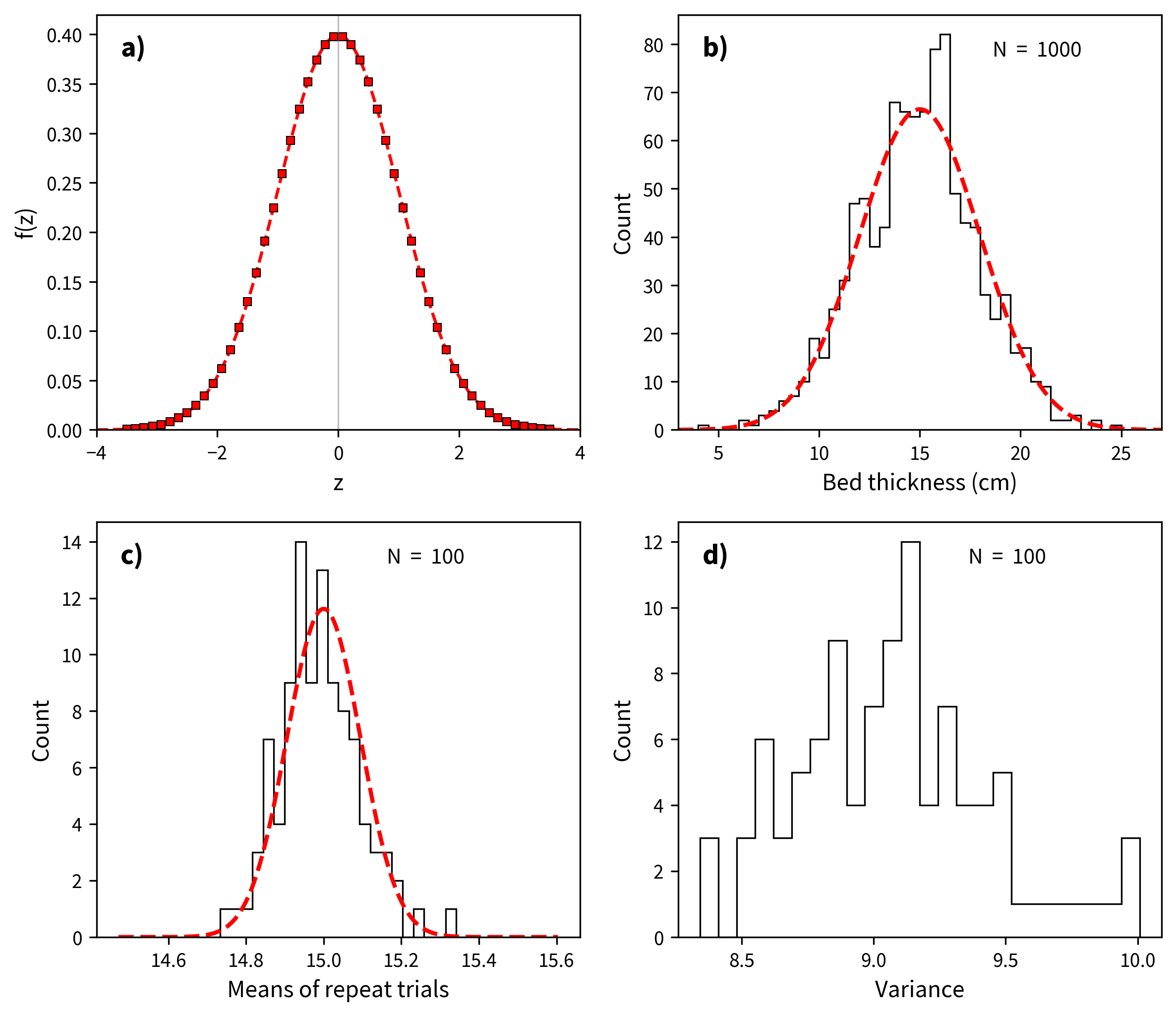
Figure 11.1:a) The Gaussian probability density function (normal distribution, Equation 11.1). The proportion of observations within an interval centered on is . b) Histogram of 1000 simulated measurements of bed thickness in a sedimentary formation, drawn from a normal distribution with a mean of 15 and a standard deviation of 3. Also shown is the smooth curve of the generating distribution. c) Histogram of the means from 100 repeated sets of 1000 measurements from the same distribution. The distribution of the means is much tighter. d) Histogram of the variances () from the same set of experiments as in c). The distribution of variances is not bell shaped; it is .
The Gaussian probability density function is given by:
where
is the variable measured, is the true mean, and is the standard deviation. The parameter determines the value of about which the distribution is centered, while determines the width of the distribution about the true mean. By performing the required integrals (computing area under curve ), it can be shown that 68% of the readings in a normal distribution are within of , while 95% are within 1.96 of .
The usual situation is that one has made a finite number of measurements of a variable . In the literature of statistics, this set of measurements is referred to as a sample. Let us say that we made 1000 measurements of some parameter, say bed thickness (in cm) in a particular sedimentary formation. We plot these in histogram form in Figure 11.1b.
By using the methods of Gaussian statistics, one is supposing that the observed sample has been drawn from a population of observations that is normally distributed. The true mean and standard deviation of the population are, of course, unknown. But the following methods allow estimation of these quantities from the observed sample. A normal distribution can be characterized by two parameters, the mean () and the variance . How to estimate the parameters of the underlying distribution is the art of statistics. We all know that the arithmetic mean of a batch of data drawn from a normal distribution is calculated by:
where is the number of measurements and is an individual measurement.
The mean estimated from the data shown in Figure 11.1b is 14.91. If we had measured an infinite number of bed thicknesses, we would have gotten the bell curve shown as the dashed line and calculated a mean of 15.
The “spread” in the data is characterized by the variance . Variance for normal distributions can be estimated by the statistic :
In order to get the units right on the spread about the mean (cm -- not cm), we have to take the square root of . The statistic gives an estimate of the standard deviation and is the bounds around the mean that includes 68% of the values. The 95% confidence bounds are given by 1.96 (this is what a “2- error” is), and should include 95% of the observations. The bell curve shown in Figure 11.1b has a (standard deviation) of 3, while the is 2.97.
If you repeat the bed measuring experiment a few times, you will never get exactly the same measurements in the different trials. The mean and standard deviations measured for each trial then are “sample” means and standard deviations. If you plotted up all those sample means, you would get another normal distribution whose mean should be pretty close to the true mean, but with a much more narrow standard deviation. In Figure 11.1c we plot a histogram of means from 100 such trials of 1000 measurements each drawn from the same distribution of . In general, we expect the standard deviation of the means (or standard error of the mean, ) to be related to by
What if we were to plot up a histogram of the estimated variances as in Figure 11.1d? Are these also normally distributed? The answer is no, because variance is a squared parameter relative to the original units. In fact, the distribution of variance estimates from normal distributions is expected to be chi-squared (). The width of the distribution is also governed by how many measurements were made. The so-called number of degrees of freedom () is given by the number of measurements made minus the number of measurements required to make the estimate, so for our case is . Therefore we expect the variance estimates to follow a distribution with degrees of freedom of .
The estimated standard error of the mean, , provides a confidence limit for the calculated mean. Of all the possible samples that can be drawn from a particular normal distribution, 95% have means, , within 2 of . (Only 5% of possible samples have means that lie farther than 2 from .) Thus, the 95% confidence limit on the calculated mean, , is 2, and we are 95% certain that the true mean of the population from which the sample was drawn lies within 2 of . The estimated standard error of the mean, , decreases as 1/. Larger samples provide more precise estimations of the true mean; this is reflected in the smaller confidence limit with increasing .
We often wish to consider ratios of variances derived from normal distributions (for example to decide if the data are more scattered in one data set relative to another). In order to do this, we must know what ratio would be expected from data sets drawn from the same distributions. Ratios of such variances follow a so-called distribution with and degrees of freedom for the two data sets. This is denoted . Thus, if the ratio , given by:
is greater than the 5% critical value of (check the F distribution tables in your favorite statistics book or online), the hypothesis that the two variances are the same can be rejected at the 95% level of confidence.
A related test to the test is Student’s -test. This test compares differences in normal data sets and provides a means for judging their significance. Given two sets of measurements of bed thickness, for example in two different sections, the test addresses the likelihood that the difference between the two means is significant at a given level of probability. If the estimated means and standard deviations of the two sets of and measurements are and respectively, the statistic can be calculated by:
where
Here . If this number is below a critical value for then the null hypothesis that the two sets of data are the same cannot be rejected at a given level of confidence. The critical value can be looked up in -tables in your favorite statistics book or online.
11.2Statistics of Vectors
We turn now to the trickier problem of sets of measured vectors. We will consider the case in which all vectors are assumed to have a length of one, i.e., these are unit vectors. Unit vectors are just “directions.” Paleomagnetic directional data are subject to a number of factors that lead to scatter. These include:
uncertainty in the measurement caused by instrument noise or specimen alignment errors,
uncertainties in sample orientation,
uncertainty in the orientation of the sampled rock unit,
variations among samples in the degree of removal of a secondary component,
uncertainty caused by the process of magnetization,
secular variation of the Earth’s magnetic field, and
lightning strikes.
Some of these sources of scatter (e.g., items 1, 2 and perhaps 6 above) lead to a symmetric distribution about a mean direction. Other sources of scatter contribute to distributions that are wider in one direction than another. For example, in the extreme case, item 4 leads to a girdle distribution whereby directions are smeared along a great circle. It would be handy to be able to calculate a mean direction for data sets and to quantify the scatter.
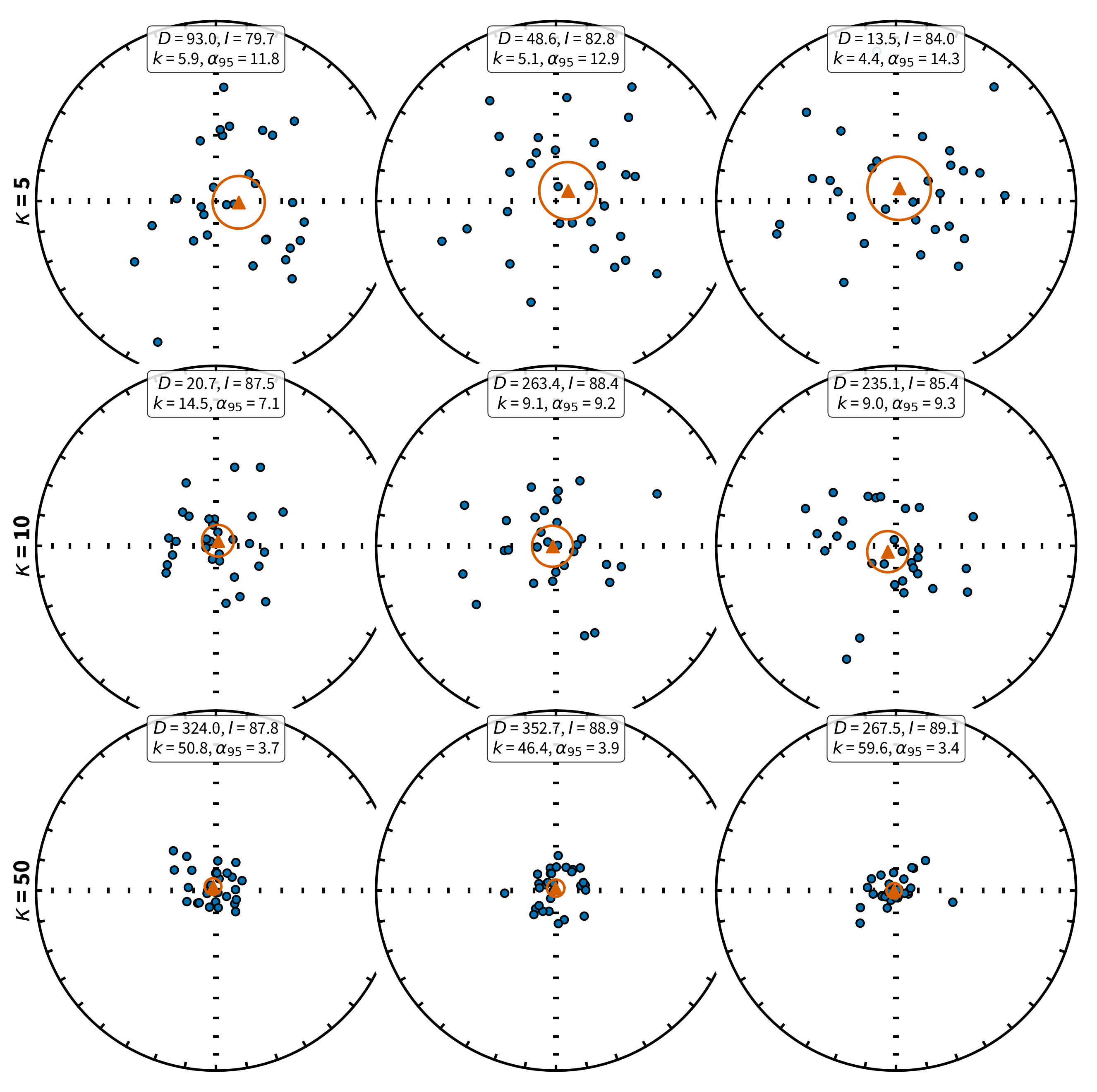
Figure 11.2:Hypothetical data sets drawn from Fisher distributions with vertical true directions. Each row shows three realizations for = 5 (top row), = 10 (middle row), and = 50 (bottom row). Estimated mean declination (), mean inclination (), precision parameter (), and 95% confidence angle () shown in insets. Blue circles are individual directions; orange triangles are the estimated mean directions with confidence circles.
In order to calculate mean directions with confidence limits, paleomagnetists rely heavily on the special statistics known as Fisher statistics Fisher (1953), which were developed for assessing dispersion of unit vectors on a sphere. It is applicable to directional data that are dispersed in a symmetric manner about the true direction. We show some examples of such data in Figure 11.2 with varying amounts of scatter from highly scattered in the top row to rather concentrated in the bottom row. All the data sets were drawn from a Fisher distribution with a vertical true direction.
In most instances, paleomagnetists assume a Fisher distribution for their data because the statistical treatment allows calculation of confidence intervals, comparison of mean directions, comparison of scatter, etc. The average inclination, calculated as the arithmetic mean of the inclinations, will never be vertical unless all the inclinations are vertical. In the following, we will demonstrate the proper way to calculate mean directions and confidence regions for directional data that are distributed in the manner shown in Figure 11.2. We will also briefly describe several useful statistical tests that are popular in the paleomagnetic literature.
11.2.1Estimation of Fisher Statistics
R. A. Fisher developed a probability density function applicable to many paleomagnetic directional data sets, known as the Fisher distribution Fisher (1953). In Fisher statistics each direction is given unit weight and is represented by a point on a sphere of unit radius. The Fisher distribution function gives the probability per unit angular area of finding a direction within an angular area, , centered at an angle from the true mean. The angular area, , is expressed in steradians, with the total angular area of a sphere being steradians. Directions are distributed according to the Fisher probability density, given by:
where is the angle between the unit vector and the true direction and is a precision parameter such that as , dispersion goes to zero.
We can see in Figure 11.3a the probability of finding a direction within an angular area centered degrees away from the true mean for different values of . is a measure of the concentration of the distribution about the true mean direction. The larger the value of , the more concentrated the direction; is 0 for a distribution of directions that is uniform over the sphere and approaches for directions concentrated at a point.
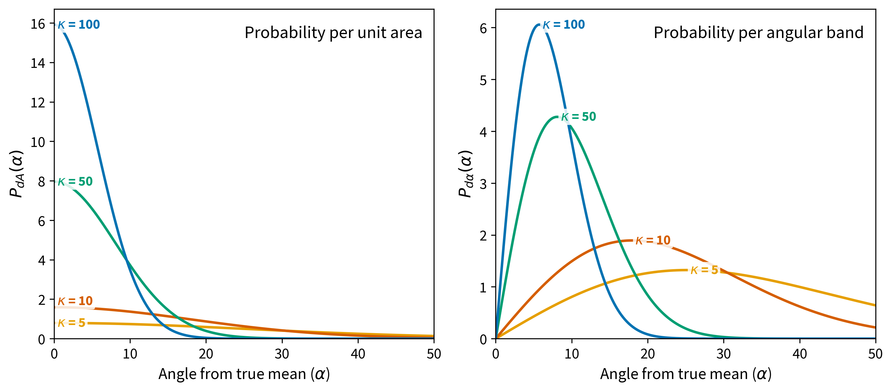
Figure 11.3:Fisher probability density functions for = 5, 10, 50, and 100. Left: probability of finding a direction within an angular area centered at angle from the true mean. Right: probability of finding a direction at angle away from the true mean direction, which includes the factor that accounts for the decreasing area of angular bands near the poles.
If is taken as the azimuthal angle about the true mean direction, the probability of a direction within an angular area, , can be expressed as
The term arises because the area of a band of width varies as . It should be understood that the Fisher distribution is normalized so that
Equation 11.11 simply indicates that the probability of finding a direction somewhere on the unit sphere must be unity. The probability of finding a direction in a band of width between and is given by:
This probability (for ) is shown in Figure 11.3b where the effect of the term is apparent. Equation 11.9 for the Fisher distribution function suggests that declinations are symmetrically distributed about the mean. In “data” coordinates, this means that the declinations are uniformly distributed from 0 360°. Furthermore, the probability of finding a direction of away from the mean decays exponentially.
Because the intensity of the magnetization has little to do with the validity of the measurement (except for very weak magnetizations), it is customary to assign unit length to all directions. The mean direction is calculated by first converting the individual moment directions () (see Figure 11.4), which may be expressed as declination and inclination (), to Cartesian coordinates () by the methods given in Chapter 2. Following the logic for vector addition explained in Section A.3.2, the length of the vector sum, or resultant vector , is given by:
The relationship of to the individual unit vectors is shown in Figure 11.4. is always and approaches only when the vectors are tightly clustered. The mean direction components are given by:
These Cartesian coordinates can, of course, be converted back to geomagnetic elements () by the familiar method described in Chapter 2.
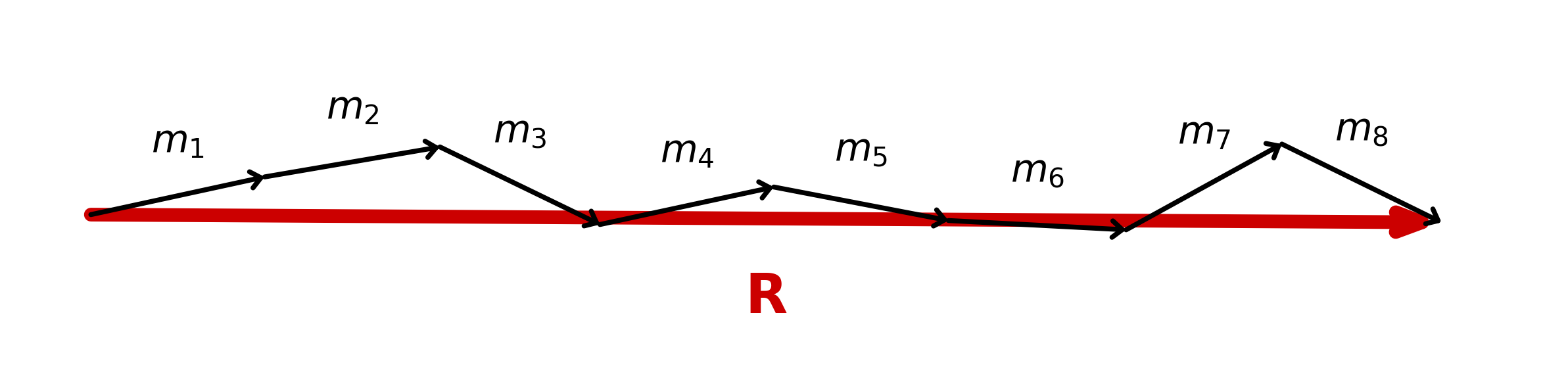
Figure 11.4:Vector addition of eight unit vectors m1 through m8 arranged head-to-tail to yield the resultant vector .
Having calculated the mean direction, the next objective is to determine a statistic that can provide a measure of the dispersion of the population of directions from which the sample data set was drawn. One measure of the dispersion of a population of directions is the precision parameter, . From a finite sample set of directions, is unknown, but a best estimate of can be calculated by
where is the number of data points. Using this estimate of , we estimate the circle of 95% confidence () about the mean, , by:
In the classic paleomagnetic literature, was further approximated by:
which is reliable for larger than about 25 (see Tauxe et al. (1991)). By direct analogy with Gaussian statistics (Equation 11.4), the angular variance of a sample set of directions is:
where is the angle between the direction and the calculated mean direction. The estimated circular (or angular) standard deviation is , which can be approximated by:
which is the circle containing ~68% of the data.
Some practitioners use the statistic given by:
because of its ease of calculation and the intuitive appeal (e.g., Figure 11.4) that decreases as approaches . In practice, when , CSD and are close to equal.
When we calculate the mean direction, a dispersion estimate, and a confidence limit, we are supposing that the observed data came from random sampling of a population of directions accurately described by the Fisher distribution. But we do not know the true mean of that Fisherian population, nor do we know its precision parameter . We can only estimate these unknown parameters. The calculated mean direction of the directional data set is the best estimate of the true mean direction, while is the best estimate of . The confidence limit is a measure of the precision with which the true mean direction has been estimated. One is 95% certain that the unknown true mean direction lies within of the calculated mean. The obvious corollary is that there is a 5% chance that the true mean lies more than from the calculated mean.
11.2.2Some Illustrations
Having buried the reader in mathematical formulations, we present the following illustrations to develop some intuitive appreciation for the statistical quantities. One essential concept is the distinction between statistical quantities calculated from a directional data set and the unknown parameters of the sampled population.
Consider the various sets of directions plotted as equal area projections in Figure 11.2. These are all synthetic data sets drawn from Fisher distributions with means of a single, vertical direction. Each of the three diagrams in a row is a replicate sample from the same distribution. The top row were all drawn from a distribution with , the middle with and the bottom row with . For each synthetic data set, we estimated and (shown as insets to the equal area diagrams).
There are several important observations to be taken from these examples. Note that the calculated mean direction is never exactly the true mean direction ( = +90°). The calculated mean inclination varies from 79.7° to 89.1°, and the mean declinations fall within all quadrants of the equal-area projection. The calculated mean direction thus randomly dances about the true mean direction and deviates from the true mean by between 0.9° and 10.3°. The calculated statistic varies considerably among replicate samples as well. The variation of and differences in angular variance of the data sets with the same underlying distribution are simply due to the vagaries of random sampling.
The confidence limit varies from 3.4° to 14.3° and is shown by the circle surrounding the calculated mean direction (shown as a triangle). For these directional data sets, none of the calculated means falls more than from the true mean. However, if 100 such synthetic data sets had been analyzed, on average five would have a calculated mean direction removed from the true mean direction by more than the calculated confidence limit . That is, the true mean direction would lie outside the circle of 95% confidence, on average, in 5% of the cases.
It is also important to appreciate which statistical quantities are fundamentally dependent upon the number of observations . Neither the value (Equation 11.16) nor the estimated angular deviation CSD (Equation 11.20) is fundamentally dependent upon . These statistical quantities are estimates of the intrinsic dispersion of directions in the Fisherian population from which the data set was sampled. Because that dispersion is not affected by the number of times the population is sampled, the calculated statistics estimating that dispersion should not depend fundamentally on the number of observations . However, the confidence limit should depend on ; the more individual measurements there are in our sample, the greater must be the precision (and accuracy) in estimating the true mean direction. This increased precision should be reflected by a decrease in with increasing . Indeed Equation 11.17 indicates that depends approximately on .
Figure 11.5 illustrates these dependencies of calculated statistics on number of directions in a data set. This diagram was constructed as follows:
We drew a synthetic data set of from a Fisher distribution with a of 29.2 (equivalent to a circular standard deviation of 15°).
Starting with the first four directions in the synthetic data set, a subset of = 4 was used to calculate , CSD and using Equations 11.16, 11.20, and 11.21 respectively. In addition, (using Equation 11.17) was calculated. Resulting values of CSD, and are shown in Figure 11.5 as a function of .
For each succeeding value of in Figure 11.5, the next direction from the = 30 synthetic data set was added to the previous subset of directions, continuing until the full = 30 synthetic data set was used.
The effects of increasing are apparent in Figure 11.5 in which we show a comparison of the two estimates of , CSD and . Although not fundamentally dependent upon , in practice the estimated angular standard deviation, CSD, deviates from for values of , only approaching the correct value when . As expected, the calculated confidence limit decreases approximately as , showing a dramatic decrease in the range and more gradual decrease for .
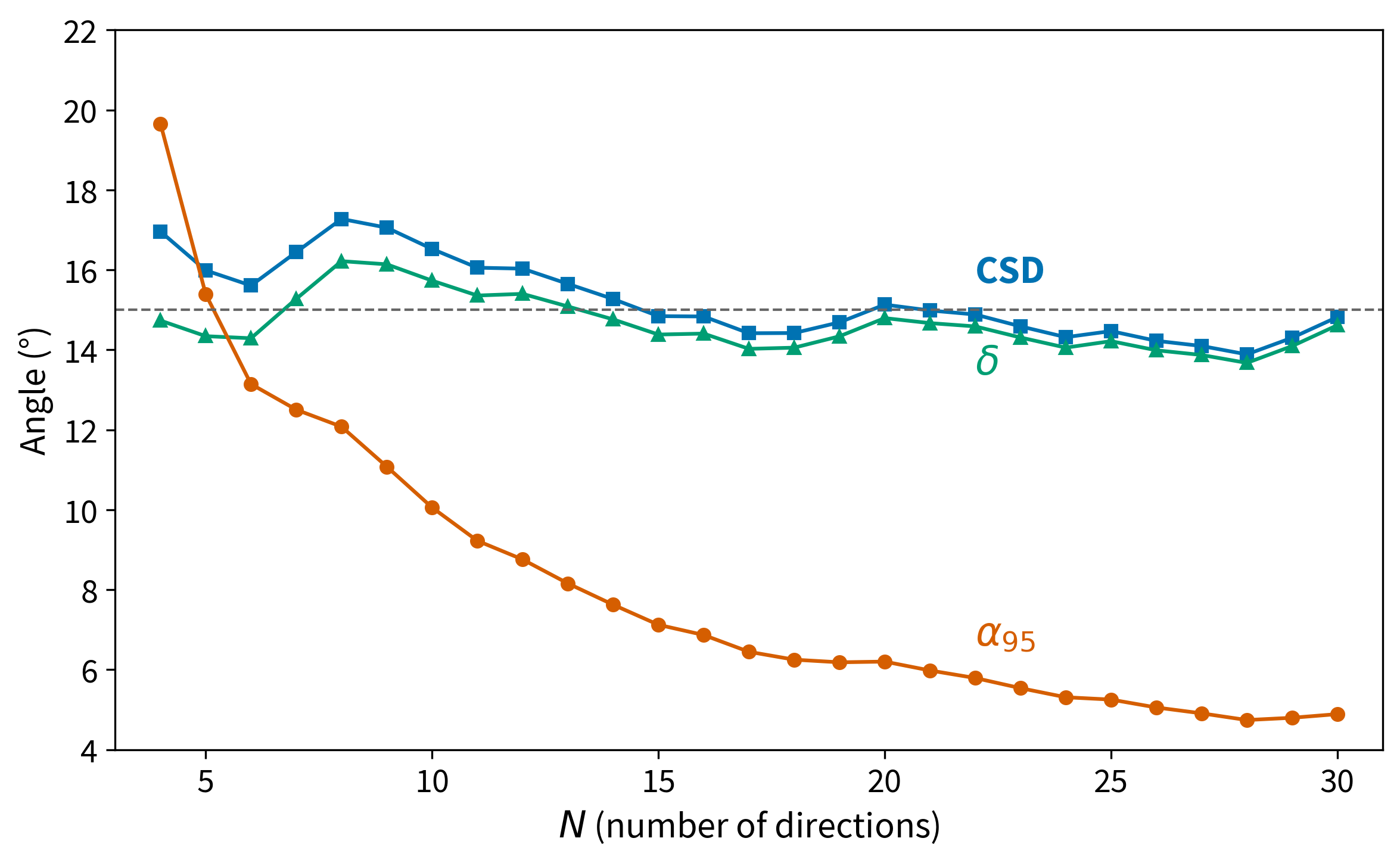
Figure 11.5:Dependence of estimated angular standard deviation, CSD and , and confidence limit, , on the number of directions in a data set. An increasing number of directions were selected from a Fisherian sample of directions with angular standard deviation = 15° ( = 29.2), shown by the horizontal line.
If directions are converted to VGPs as outlined in Chapter 2, the transformation distorts a rotationally symmetric set of data into an elliptical distribution. The associated may no longer be appropriate. Cox & Doell (1960) suggested the following for 95% confidence regions in VGPs. Ironically, it is more likely that the VGPs are spherically symmetric, implying that most sets of directions are not!
where is the semi-axis parallel to the meridians (lines of longitude), is the semi-axis parallel to the parallels (lines of latitude), and is the site paleolatitude.
11.3Significance Tests
The Fisher distribution allows us to ask a number of questions about paleomagnetic data sets, such as:
Is a given set of directions random? This is the question that we ask when we perform a conglomerate test (Chapter 9).
Is one data set better grouped than another as in the fold test from Chapter 9?
Is the mean direction of a given (Fisherian) data set different from some known direction? This question comes up when we compare a given data set with, for example, the directions of the present or GAD field.
Are two (Fisherian) data sets different from each other? For example, are the normal directions and the antipodes of the reversed directions the same for a given data set?
If a given site has some samples that allow only the calculation of a best-fit plane and not a directed line, what is the site mean direction that combines the best-fit lines and planes (see Chapter 9)?
In the following discussion, we will briefly summarize ways of addressing these issues using Fisher techniques. There are two fundamental principles of statistical significance tests that are important to the proper interpretation:
Tests are generally made by comparing an observed sample with a null hypothesis. For example, in comparing two mean paleomagnetic directions, the null hypothesis is that the two mean directions are separate samples from the same population of directions. (This is the same as saying that the samples were not, in fact, drawn from different populations with distinct true mean directions.) Significance tests do not disprove a null hypothesis but only show that observed differences between the sample and the null hypothesis are unlikely to have occurred because of sampling limitations. In other words, there is probably a real difference between the sample and the null hypothesis, indicating that the null hypothesis is probably incorrect.
Any significance test must be applied by using a level of significance. This is the probability level at which the differences between a set of observations and the null hypothesis may have occurred by chance. A commonly used significance level is 5%. In Gaussian statistics, when testing an observed sample mean against a hypothetical population mean (the null hypothesis), there is only a 5% chance that is more than 2 from the mean, , of the sample. If differs from by more than 2, is said to be “statistically different from at the 5% level of significance,” using proper statistical terminology. However, the corollary of the actual significance test is often what is reported by statements such as “ is distinct from at the 95% confidence level.” The context usually makes the intended meaning clear, but be careful to practice safe statistics.
An important sidelight to this discussion of level of significance is that too much emphasis is often put on the 5% level of significance as a magic number. Remember that we are often performing significance tests on data sets with a small number of observations. Failure of a significance test at the 5% level of significance means only that the observed differences between sample and null hypothesis cannot be shown to have a probability of chance occurrence that is > 5%. This does not mean that the observed differences are unimportant. Indeed the observed differences might be significant at a marginally higher level of significance (for instance, 10%) and might be important to the objective of the paleomagnetic investigation.
Significance tests for use in paleomagnetism were developed in the 1950s by G.S. Watson and E.A. Irving. These versions of the significance tests are fairly simple, and an intuitive appreciation of the tests can be developed through a few examples. Because of their simplicity and intuitive appeal, we investigate these “traditional” significance tests in the development below. However, many of these tests have been updated using advances in statistical sampling theory. These will be discussed in Chapter 12. While they are technically superior to the traditional significance tests, they are more complex and less intuitive than the traditional tests.
11.3.1Watson’s Test for Randomness
Watson (1956) demonstrated how to test a given directional data set for randomness. His test relies on the calculation of given by Equation 11.14. Because is the length of the resultant vector, randomly directed vectors will have small values of , while, for less scattered directions, will approach . Watson (1956) defined a parameter that can be used for testing the randomness of a given data set. If the value of exceeds , the null hypothesis of total randomness can be rejected at a specified level of confidence. If is less than , randomness cannot be rejected. Watson calculated the value of for a range of for the 95% and 99% confidence levels. Watson (1956) also showed how to estimate by:
The estimation works well for , but is somewhat biased for smaller data sets. The critical values of for from Watson (1956) are listed for convenience in Table 11.1.
The test for randomness is particularly useful for determining if, for example, the directions from a given site are randomly oriented (the data for the site should therefore be thrown out). Also, one can determine if directions from the conglomerate test are random or not (see Chapter 9).
11.3.2Comparison of Precision
In the fold test (or bedding-tilt test), one examines the clustering of directions before and after performing structural corrections. If the clustering improves on structural correction, the conclusion is that the ChRM was acquired prior to folding and therefore “passes the fold test”. The appropriate significance test determines whether the improvement in clustering is statistically significant. Here we will discuss a very quick, back-of-the-envelope test for this proposed by McElhinny (1964). This form of the fold test is not used much anymore (see McFadden & Jones (1981)), but serves as a quick and intuitively straight-forward introduction to the subject.
Consider two directional data sets, one with directions and , and one with directions and . If we assume (null hypothesis) that these two data sets are samples of populations with the same , the ratio is expected to vary because of sampling errors according to
where and are variances with and degrees of freedom. This ratio should follow the -distribution if the assumption of common is correct. Fundamentally, one expects this ratio to be near 1.0 if the two samples were, in fact, selections from populations with common . The -distribution tables indicate how far removed from 1.0 the ratio may be before the deviation is significant at a chosen probability level. If the observed ratio in Equation 11.24 is far removed from 1.0, then it is highly unlikely that the two data sets are samples of populations with the same . In that case, the conclusion is that the difference in the values is significant and the two data sets were most likely sampled from populations with different .
As applied to the fold test, one examines the ratio of after tectonic correction () to before tectonic correction (). The significance test for comparison of precisions determines whether is significantly removed from 1.0. If exceeds the value of the -distribution for the 5% significance level, there is less than a 5% chance that the observed increase in resulting from the tectonic correction is due only to sampling errors. There is 95% probability that the increase in is meaningful and the data set after tectonic correction is a sample of a population with larger than the population sampled before tectonic correction. Such a result constitutes a “statistically significant passage of the fold test.”
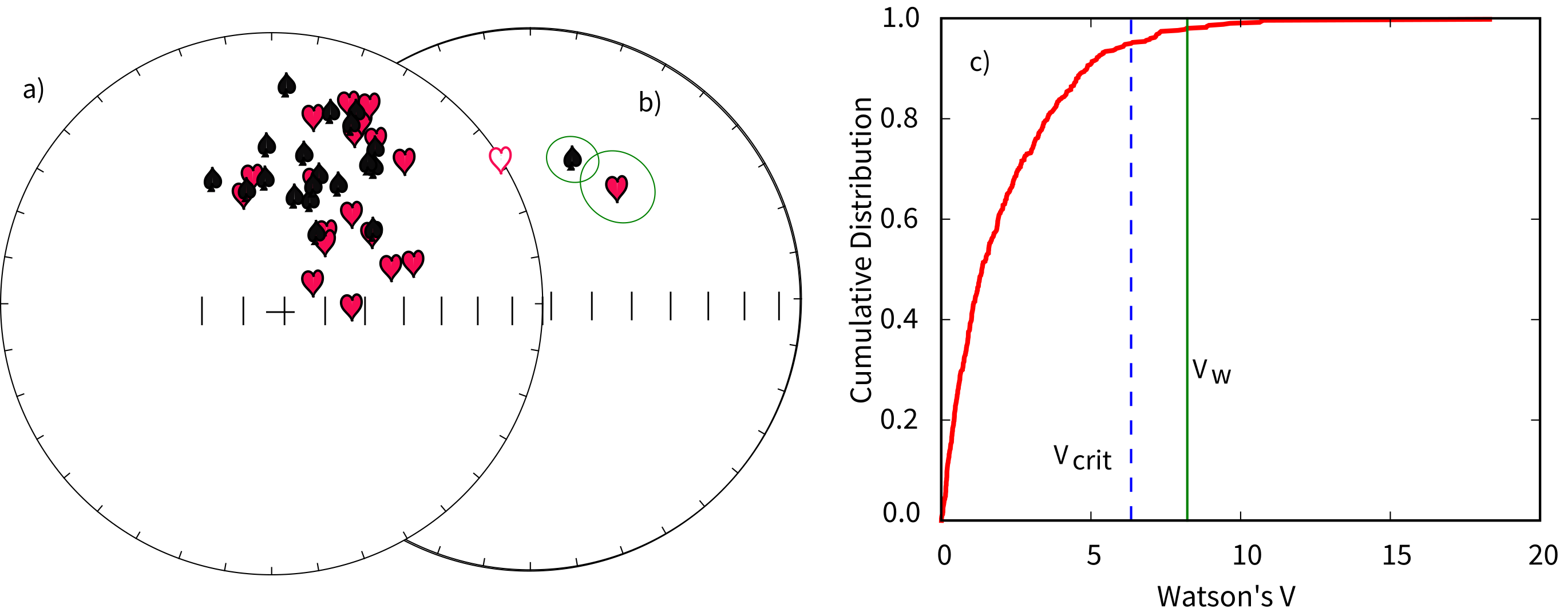
Figure 11.6:a) Equal area projections of declinations and inclinations of two hypothetical data sets. b) Fisher means and circles of confidence from the data sets in a). c) Distribution of for simulated Fisher distributions with the same and as the two shown in a). The dashed line is the upper bound for the smallest 95% of the s calculated for the simulations (). The solid vertical line is the calculated for the two data sets. According to this test, the two data sets do not have a common mean, despite their overlapping confidence ellipses.
11.3.3Comparing Known and Estimated Directions
The calculation of confidence regions for paleomagnetic data is largely motivated by a need to compare estimated directions with either a known direction (for example, the present field) or another estimated direction (for example, that expected for a particular paleopole, the present field or a GAD field). Comparison of a paleomagnetic data set with a given direction is straight-forward using Fisher statistics. If the known test direction lies outside the confidence interval computed for the estimated direction, then the estimated and known directions are different at the specified confidence level.
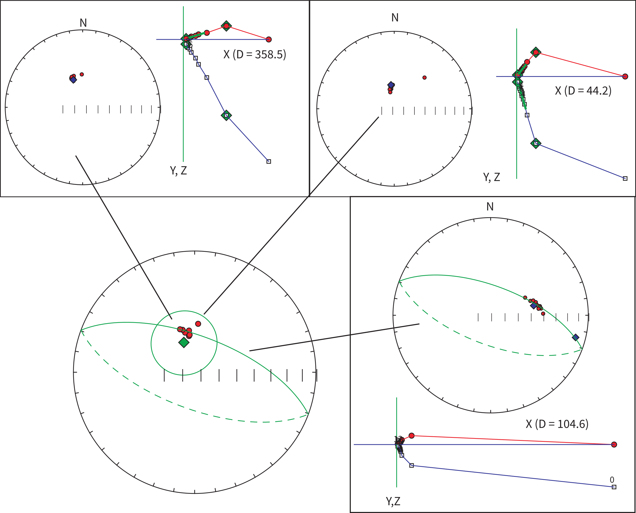
Figure 11.7:Examples of demagnetization data from a site whose mean is partially constrained by a great circle. The best-fit great circle and six directed lines allow a mean (diamond) and associated to be calculated using the method of McFadden & McElhinny (1988). Demagnetization data for two of the directed lines are shown at the top of the diagram while those for the great circle are shown at the bottom. [Data from Tauxe et al. (2004).]
11.3.4Comparing Two Estimated Directions
The case in which we are comparing two Fisher distributions can also be relatively straight forward. If the two confidence circles do not overlap, the two directions are different at the specified (or more stringent) level of certainty. When one confidence region includes the mean of the other set of directions, the difference in directions is not significant.
The situation becomes a little more tricky when the data sets are as shown in Figure 11.6a. The Fisher statistics for the two data sets are:
| symbol | |||||||
|---|---|---|---|---|---|---|---|
| 1 | spades | 38.0 | 45.7 | 20 | 18.0818 | 9.9 | 10.9 |
| 2 | hearts | 16.9 | 45.2 | 20 | 19.0899 | 20.9 | 7.3 |
As shown in the equal area projection in Figure 11.6b, the two s overlap, but neither includes the mean of the other. This sort of “grey zone” case has been addressed by many workers.
The most common way of testing the significance of two sets of directions is a simple test, proposed by Watson (1956). Consider two directional data sets: one has directions (described by unit vectors) yielding a resultant vector of length ; the other has directions yielding resultant . The statistic
must be determined, where and is the resultant of all individual directions. This statistic is compared with tabulated values for 2 and 2(-2) degrees of freedom. If the observed statistic exceeds the tabulated value at the chosen significance level, then these two mean directions are different at that level of significance.
The tabulated -distribution indicates how different two sample mean directions can be (at a chosen probability level) because of sampling errors. If the calculated mean directions are very different but the individual directional data sets are well grouped, intuition tells us that these mean directions are distinct. The mathematics described above should confirm this intuitive result. With two well-grouped directional data sets with very different means, , , and , so that . With these conditions, the statistic given by Equation 11.25 will be large and will easily exceed the tabulated value. So this simple intuitive examination of Equation 11.25 yields a sensible result.
An alternative, and in many ways superior, statistic () was proposed by Watson (1983) (see Section C.2.1 for details). was posed as a test statistic that increases with increasing difference between the mean directions of the two data sets. Thus, the null hypothesis that two data sets have a common mean direction can be rejected if exceeds some critical value which can be determined through what is called Monte Carlo simulation. The technique gets its name from a famous gambling locale because we use randomly drawn samples (“cards”) from specified distributions (“decks”) to see what can be expected from chance. What we want to know is the probability that two data sets (hands of cards?) drawn from the same underlying distribution would have a given statistic just from chance.
We proceed as follows:
Calculate the statistic for the data sets. [The for the two data sets shown in Figure 11.6a is 8.5.]
In order to determine the critical value for , we draw two Fisher distributed data sets with dispersions of and and , but having a common true direction.
We then calculate for these simulated data sets.
Repeat the simulation some large number of times (say 1000). This defines the distribution of s that you would get from chance by “sampling” distributions with the same direction.
Sort the s in order of increasing size. The critical value of at the 95% level of confidence is the 950 simulated .
The s simulated for two distributions with the same and as our example data sets but drawn from distributions with the same mean are plotted as a cumulative distribution function in Figure 11.6c with the bound containing the lowermost 95% of the simulations shown as a dashed line at 6.2. The value of 8.5, calculated for the data set is shown as a heavy vertical line and is clearly larger than 95% of the simulated populations. This simulation therefore supports the suggestion that the two data sets do not have a common mean at the 95% level of confidence.
This test can be applied to the two polarities in a given data collection to see if they are antipodal. In this case, one would take the antipodes of one of the data sets before calculating . Such a test would be a Fisherian form of the reversals test.
11.3.5Combining Directions and Great Circles
Consider the demagnetization data shown in Figure 11.7 of various specimens from a certain site. Best-fit lines from the data for the two specimens at the top of the diagram are calculated using principal component analysis (Chapter 9). The data from the specimen shown at the bottom of the diagram track along a great circle path and can be used to find the pole to the best-fit plane calculated also as in Chapter 9. McFadden & McElhinny (1988) described a method for estimating the mean direction (diamond in central equal area plot) and the from sites that mixes planes (great circles on an equal area projection) and directed lines (see Section C.2.2). The key to their method is to find the direction within each plane that gives the tightest grouping of directions. Then “regular” Fisher statistics can be applied.
11.4Inclination Only Data
A different problem arises when only the inclination data are available as in the case of unoriented drill cores. Cores can be drilled and arrive at the surface in short, unoriented pieces. Specimens taken from such core material will be oriented with respect to the vertical, but the declination data are unknown. It is often desirable to estimate the true Fisher inclination of data sets having only inclination data, but how to do this is not obvious. Consider the data in Figure 11.8. The true Fisher mean declination and inclination are shown by the triangle. If we had only the inclination data and calculated a Gaussian mean (), the estimate would be too shallow as pointed out earlier.
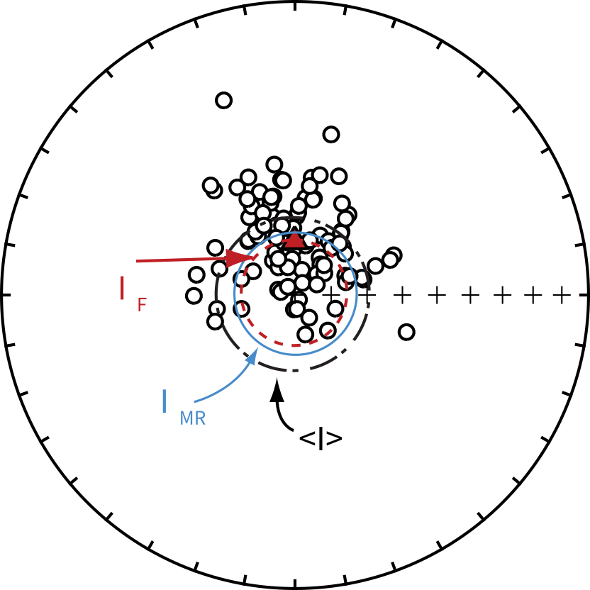
Figure 11.8:Directions drawn from a Fisher distribution with a near vertical true mean direction. The Fisher mean direction from the sample is shown by the triangle. The Gaussian average inclination () is shallower than the Fisher mean . The estimated inclination using the maximum likelihood estimate of McFadden & Reid (1982) () is closer to the Fisher mean than the Gaussian average.
Several investigators have addressed the issue of inclination-only data. McFadden & Reid (1982) developed a maximum likelihood estimate for the true inclination which works reasonably well. Their approach is outlined in Appendix F.
By comparing inclinations estimated using the McFadden-Reid technique with those calculated using the full vector data, it is clear that the method breaks down at high inclinations and high scatter. It is also inappropriate for data sets that are not Fisher distributed!
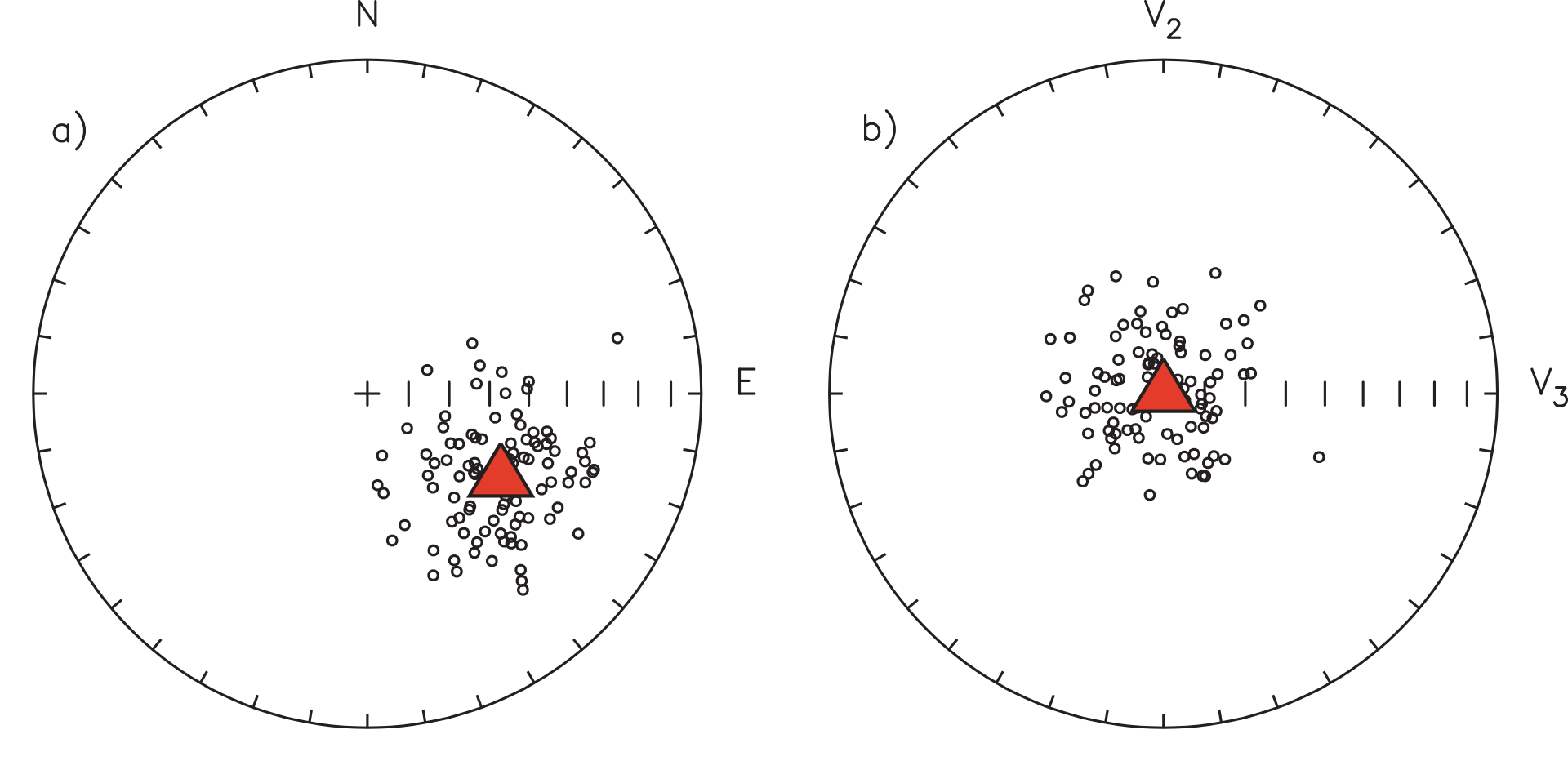
Figure 11.9:Transformation of coordinates from a) geographic to b) “data” coordinates. The direction of the principal eigenvector is shown by the triangle in both plots. [Figure redrawn from Tauxe (1998).]
11.5Is a Given Data Set Fisher Distributed?
Clearly, the Fisher distribution allows powerful tests and this power lies behind the popularity of paleomagnetism in solving geologic problems. The problem is that these tests require that the data be Fisher distributed. How can we tell if a particular data set is Fisher distributed? What do we do if the data are not Fisher distributed? These questions are addressed in the rest of this chapter and the next one.
Let us now consider how to determine whether a given data set is Fisher distributed. There are actually many ways of doing this. There is a rather complete discussion of the problem in Fisher et al. (1987) and if you really want a complete treatment try the supplemental reading list at the end of this chapter. The quantile-quantile (Q-Q) method described by Fisher et al. (1987) is fairly intuitive and works well. We outline it briefly in the following.
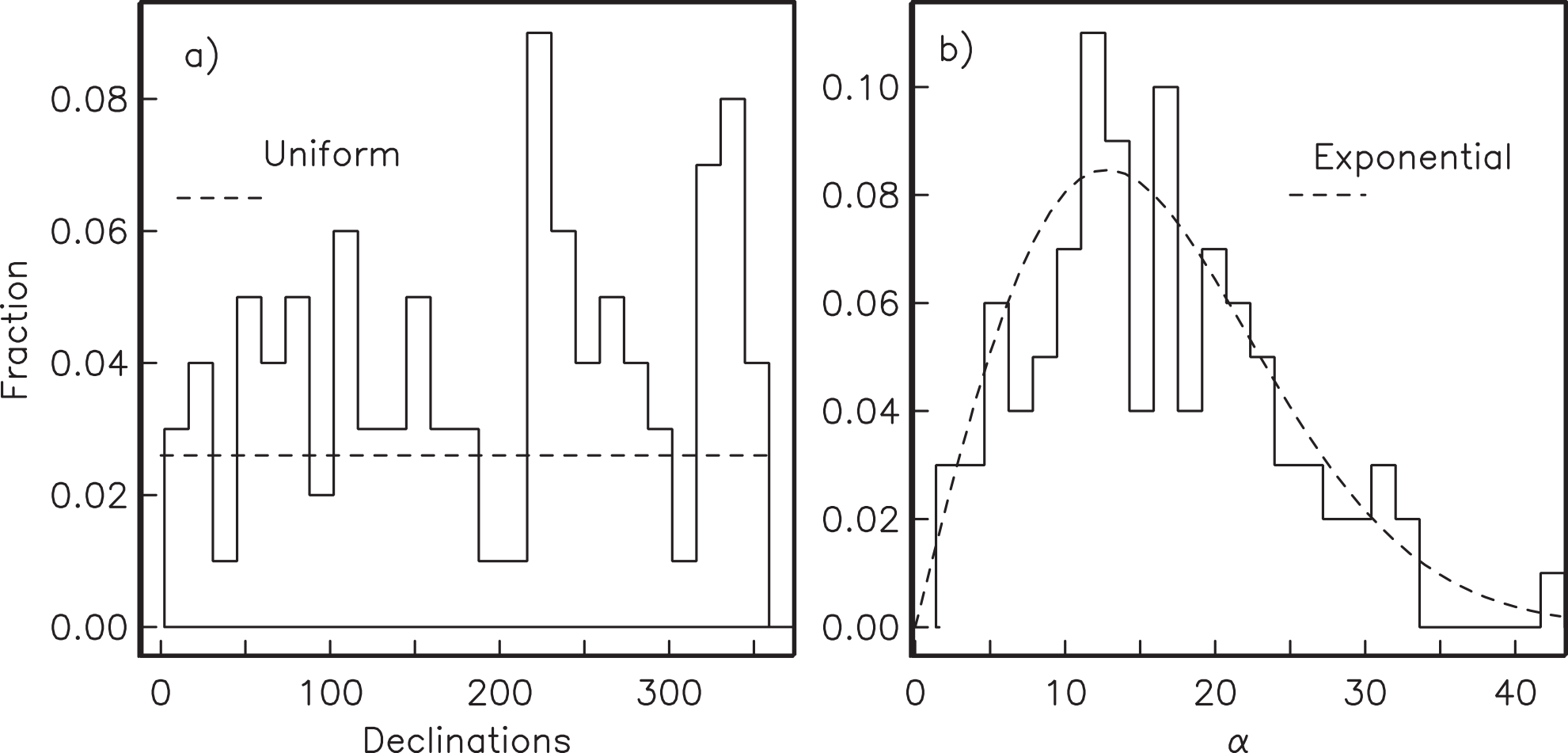
Figure 11.10:a) Declinations and b) co-inclinations () from Figure 11.9. Also shown are behaviors expected for and from a Fisher distribution, i.e., declinations are uniformly distributed while co-inclinations are exponentially distributed. [Figure from Tauxe (1998).]
The idea behind the Q-Q method is to exploit the fact that declinations in a Fisher distribution, when viewed about the mean, are spread around the clock evenly -- there is a uniform distribution of declinations. Also, the inclinations (or rather the co-inclinations) are clustered close to the mean and the frequency dies off exponentially away from the mean direction.
Therefore, the first step in testing for compatibility with a Fisher distribution is to transpose the data such that the mean is the center of the distribution. You can think of this as rotating your head around to peer down the mean direction. On an equal area projection, the center of the diagram will now be the mean direction instead of the vertical. In order to do this transformation, we first calculate the orientation matrix of the data and the associated eigenvectors and eigenvalues (Section A.3.5.4 - in case you haven’t read it yet, do so now). Substituting the direction cosines relating the geographic coordinate system to the coordinate system defined by , the eigenvectors, where is the “old” and is the “new” set of axes, we can transform the coordinate system for a set of data from “geographic” coordinates (Figure 11.9a) where the vertical axis is the center of the diagram, to the “data” coordinate system, (Figure 11.9b) where the principal eigenvector () lies at the center of the diagram, after transformation into “data” coordinates.
Recalling that Fisher distributions are symmetrically disposed about the mean direction, but fall off exponentially away from that direction, let us compare the data from Figure 11.9 to the expected distributions for a Fisher distribution with (Figure 11.10). The data were generated using the program fisher.py in the PmagPy software distribution which relies on the method outlined by Fisher et al. (1987), that draws directions from a Fisher distribution with a specified . We used a of 20, and it should come as no surprise that the data fit the expected distribution rather well. But how well is “well” and how can we tell when a data set fails to be fit by a Fisher distribution?
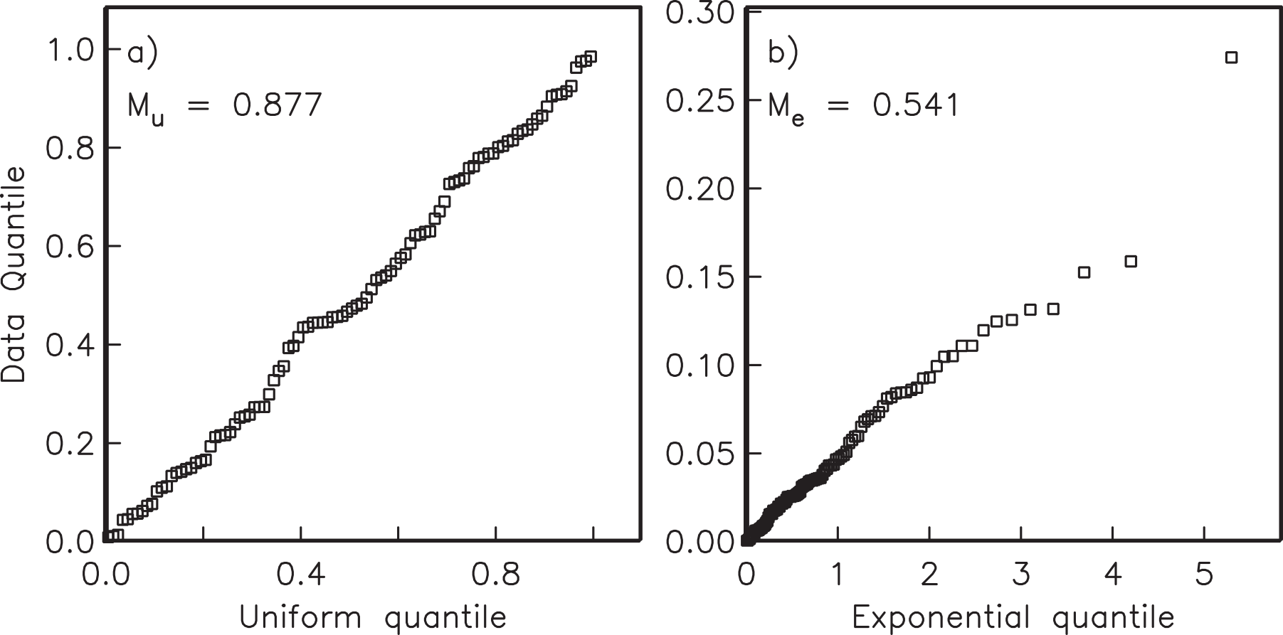
Figure 11.11:a) Quantile-quantile plot of declinations (in data coordinates) from Figure 11.9 plotted against an assumed uniform distribution. b) Same for inclinations plotted against an assumed exponential distribution. The data are Fisher distributed. [Figure from Tauxe (1998).]
We wish to test whether the declinations are uniformly distributed and whether the inclinations are exponentially distributed as required by the Fisher distribution. Plots such as those shown in Figure 11.10 are not as helpful for this purpose as a plot known as a quantile-quantile (Q-Q) diagram (see Fisher et al. (1987)). In a Q-Q plot, the data are graphed against the value expected from a particular distribution. Data compatible with the chosen distribution plot along a line. The procedure for accomplishing this is given in Section B.1.5. In Figure 11.11a, we plot the declinations from Figure 11.9 (in data coordinates) against the values calculated assuming a uniform distribution and in Figure 11.11b, we plot the co-inclinations against those calculated using an exponential distribution. As expected, the data plot along lines. Section B.1.5 outlines the calculation of two test statistics and which can be used to assess whether the data are uniformly or exponentially distributed respectively. Neither of these exceed the critical values.
11.6Problems
Review the instructions in the Preface for using PmagPy modules in Jupyter notebooks.
Problem 1
a) Use the function ipmag.fishrot to generate a Fisher distributed data set of data points, drawn from a true mean direction of , and a of 25. Use ipmag.plot_net and ipmag.plot_di to admire your handiwork.
b) Write a program to calculate the Fisher mean declination and inclination and these Fisher statistics: and CSD for the data generated in Problem 1a. You can check your answer with the PmagPy program ipmag.fisher_mean designed to work within Jupyter notebooks.
c) Generate a second sample from the same distribution (just repeat the ipmag.fishrot calls). Now you have two sets of directions drawn from the same distribution and certainly should share a common mean direction (logically). But do the two data sets pass the simple Watson’s test for common mean direction? [This test should fail 5% of the time!] Write a simple program to read in the two data files and calculate Watson’s . Check your answer using the function pmag.watsons_f.
d) Generate a third sample from a distribution with but the same and . Does this data set pass the test for common mean with the first data set in Problem 1a?
e) An alternative method for testing for common mean with less restrictive assumptions uses Watson’s statistic . Use the program ipmag.common_mean_watson to test the Problem 1a data set against the one generated in Problem 1d. Do the answers using agree with those using the test?
Problem 2
a) Draw a set of directions from a Fisher distribution with a true mean inclination of 50° (using e.g., ipmag.fishrot), an of 20 and a of 20. Calculate the Gaussian mean of the inclination data.
b) How does the Gaussian average compare with the average you calculate using your Fisher program (or ipmag.fisher_mean)?
c) Call the function pmag.doincfish, which does the inclination only calculation of . Is this estimate closer to the Fisher estimate?
Problem 3
a) Unpack the Chapter_11 datafile from the data_files archive (see the Preface for instructions). You will find a file called prob3a.dat. This has: , dip direction and dip from two limbs of the fold. They are of both polarities. Separate the data into normal and reverse polarity, flip the reverse data over to their antipodes and calculate the Fisher statistics for the combined data set.
To split the data into two modes, use the program pmag.doprinc to calculate the principal direction. Directions with an angle less than 90° away from this are in one mode and greater than 90° away are in the other. You can use Python’s Pandas filtering power for this, but you will have to write a small function to calculate the angle. For this, remember that the cosine of the angle is the dot product of the two unit vectors. Or, use pmag.angle which does just that!
Take the antipodes of one of the two sets and ‘flip’ them by adding 180 (using modulo 360! - %360) and taking the opposite of the inclination.
Calculate the means using one of the options described in Problem 1.
b) Use the function pmag.dotilt to “untilt” the data. Repeat the procedure in a). Would the two data sets pass a simple (McElhinny test) fold test?
11.7Supplemental Tables
Table 11.1:Critical values of for Watson’s test for randomness at the 95% confidence level (from Watson, 1956).
| (95%) | |
|---|---|
| 5 | 3.04 |
| 6 | 3.35 |
| 7 | 3.63 |
| 8 | 3.89 |
| 9 | 4.12 |
| 10 | 4.34 |
| 11 | 4.54 |
| 12 | 4.73 |
| 13 | 4.91 |
| 14 | 5.08 |
| 15 | 5.24 |
| 16 | 5.40 |
| 17 | 5.55 |
| 18 | 5.69 |
| 19 | 5.83 |
| 20 | 5.96 |
- Taylor, J. R. (1982). An Introduction to Error Analysis: The Study of Uncertainties in Physical Measurements. University Science Books.
- Fisher, R. A. (1953). Dispersion on a sphere. Proceedings of the Royal Society of London A, 217(1130), 295–305. 10.1098/rspa.1953.0064
- Tauxe, L., Kylstra, N., & Constable, C. G. (1991). Bootstrap statistics for paleomagnetic data. Journal of Geophysical Research: Solid Earth, 96(B7), 11723–11740. 10.1029/91JB00572
- Cox, A., & Doell, R. R. (1960). Review of paleomagnetism. Geological Society of America Bulletin, 71(6), 645–768. https://doi.org/10.1130/0016-7606(1960)71[645:ROP]2.0.CO;2
- Watson, G. S. (1956). A test for randomness of directions. Geophysical Supplements to the Monthly Notices of the Royal Astronomical Society, 7(4), 160–161. 10.1111/j.1365-246X.1956.tb05561.x
- McElhinny, M. W. (1964). Statistical significance of the fold test in palaeomagnetism. Geophysical Journal of the Royal Astronomical Society, 8(3), 338–340. 10.1111/j.1365-246X.1964.tb06300.x
- McFadden, P. L., & Jones, D. L. (1981). The fold test in palaeomagnetism. Geophysical Journal of the Royal Astronomical Society, 67(1), 53–58. 10.1111/j.1365-246X.1981.tb02731.x
- McFadden, P. L., & McElhinny, M. W. (1988). The combined analysis of remagnetization circles and direct observations in palaeomagnetism. Earth and Planetary Science Letters, 87(1–2), 161–172. 10.1016/0012-821X(88)90072-6
- Tauxe, L., Gans, P., & Mankinen, E. A. (2004). Paleomagnetism and 40Ar/39Ar ages from volcanics extruded during the Matuyama and Brunhes Chrons near McMurdo Sound, Antarctica. Geochemistry, Geophysics, Geosystems, 5(6), Q06H12. 10.1029/2003GC000656
- Watson, G. S. (1956). Analysis of dispersion on a sphere. Geophysical Supplements to the Monthly Notices of the Royal Astronomical Society, 7(4), 153–159. 10.1111/j.1365-246X.1956.tb05560.x
- Watson, G. S. (1983). Statistics on Spheres (Vol. 6). Wiley-Interscience.
- McFadden, P. L., & Reid, A. B. (1982). Analysis of palaeomagnetic inclination data. Geophysical Journal of the Royal Astronomical Society, 69(2), 307–319. 10.1111/j.1365-246X.1982.tb04950.x
- Tauxe, L. (1998). Paleomagnetic Principles and Practice. Kluwer Academic Publishers.
- Fisher, N. I., Lewis, T., & Embleton, B. J. J. (1987). Statistical Analysis of Spherical Data. Cambridge University Press. 10.1017/CBO9780511623059