Paleomagnetism is famous for its use of a large number of incomprehensible acronyms. Here we have them gathered together along with definitions and the Section numbers where they are explained in more detail. You will find here a table of physical constants and paleomagnetic parameters used in the text as well as a table listing common statistics used in paleomagnetism. After the tables, there are a few sections with useful mathematical tricks.
A.1Definitions
Table A.1:Acronyms in paleomagnetism.
| Acronym | Definition: Section # |
|---|---|
| AMS | Anisotropy of magnetic susceptibility: Section 13.1 |
| APWP | Apparent polar wander path: Section 16.2 |
| AF | Alternating field demagnetization: Section 9.1.4 |
| ARM | Anhysteretic remanent magnetization: Section 7.10 |
| ChRM | Characteristic remanent magnetization: Section 9.1.5 |
| CNS | Cretaceous Normal Superchron: Section 15.1 |
| CRM | Chemical remanent magnetization: Section 7.5 |
| DGRF | Definitive geomagnetic reference field: Section 2.2 |
| DRM | Detrital remanent magnetization: Section 7.6 |
| E/I | Elongation/inclination correction method: Section 16.4 |
| FC | Field cooled: Section 8.8.4 |
| GAD | Geocentric axial dipole: Section 2.3 |
| GHA | Greenwich hour angle: Section A.3.8 |
| GPTS | Geomagnetic polarity time scale: Chapter 15 |
| GRM | Gyroremanent magnetization: Section 7.10 |
| IGRF | International geomagnetic reference field: Section 2.2 |
| IZZI | Infield-zero field/ zero field-infield paleointensity protocol: Section 10.1.1.1 |
| IRM | Isothermal remanent magnetization: Section 5.2.1 and Section 7.7 |
| MD | Multidomain: Chapter 4 |
| MDF | Median destructive field: Section 8.2 |
| MDT | Median destructive temperature: Section 8.2 |
| NRM | Natural remanent magnetization: Chapter 7 |
| pARM | Partial anhysteretic remanence: Section 7.10 |
| pDRM | Post-depositional detrital remanent magnetization: Section 7.6 |
| PSD | Pseudo-single domain: Chapter 4 |
| PSV | Paleosecular variation of the geomagnetic field: Section 14.1 |
| pTRM | Partial thermal remanence: Section 7.4 |
| sIRM | Saturation IRM: See |
| SD | Single domain: Chapter 4 |
| SP | Superparamagnetic: Section 4.3 |
| SV | Secular variation: Section 14.1 |
| TRM | Thermal remanent magnetization: Section 7.4 |
| VADM | Virtual axial dipole moment: Section 2.4.3 |
| VDM | Virtual dipole moment: Section 2.4.3; Equation 2.21 |
| VDS | Vector difference sum: Section 9.1.6 |
| VGP | Virtual geomagnetic pole: Section 2.4.2 |
| VRM | Viscous remanent magnetization: Section 7.3 |
| SQUID | Superconducting quantum interference device: Section 9.1.2 |
| UT | Universal time (Greenwich mean time): Section A.3.8 |
| ZFC | Zero-field cooled: Section 8.8.4 |
Table A.2:Physical Parameters and Constants.
| Symbol | Definition: Section # |
|---|---|
| Magnetic susceptibility: The slope relating induced magnetization to an applied field: Section 1.5 | |
| ARM susceptibility: Section 8.6 | |
| Bulk magnetic susceptibility: Section 1.5; Equation 1.4 | |
| Diamagnetic susceptibility: Section 3.2.1 | |
| Ferromagnetic susceptibility: Section 3.3 | |
| Frequency dependent: Section 8.3.3 | |
| High-frequency susceptibility: Section 8.8.2 | |
| High-field susceptibility: Section 5.2.2 | |
| Initial susceptibility: Section 5.2.2 | |
| Low-frequency susceptibility: Section 8.8.2 | |
| Paramagnetic susceptibility: Section 3.2.2 | |
| Verwey transition temperature jump while cooling in a field: Section 8.8.4 | |
| Verwey transition temperature jump while cooling in zero field: Section 8.8.4 | |
| curve | Curve defined by subtracting the ascending from the descending curves in a hysteresis loop: Section 5.2.1 |
| Latitude, Longitude | |
| Permeability of free space: (4 x 10 Hm): Section 1.6 | |
| Relaxation time: Section 4.3; Equation 4.18 | |
| Magnetic co-latitude: Section 2.4; Equation 2.13 | |
| Co-latitude: Section 1.8 | |
| Direction cosines: Section A.3.5.1 | |
| Magnetic activity: Section 10.1.2 | |
| The radius of the Earth (6.371 x 10 m): Section 2.2 | |
| Magnetic induction: Section 1.3 | |
| Frequency factor (10 s): Section 4.3 | |
| Declination: Section 2.1; Equation 2.4 | |
| Elongation: Table 8.1 | |
| Inclination: Section 2.1; Equation 2.4 | |
| Gauss coefficients: Section 2.2 | |
| Magnetic field: Section 1.1 | |
| Coercivity of remanence; field required to reduce saturation IRM to zero: Section 5.1 | |
| Coercivity; the magnetic field required to change the magnetic moment of a particle from one easy axis to another: Section 5.1 | |
| Boltzmann’s constant (1.381 x 10 JK): Section 3.2.2 | |
| AMS measurement: Section D.1 | |
| Constant of uniaxial anisotropy energy: Paragraph and Section 4.1.5 | |
| Magnetic moment: Section 1.2 | |
| Bohr magneton (9.27 x 10 Am): Section 3.1 | |
| Magnetization: Section 1.5 | |
| Equilibrium magnetization: Section 7.3 | |
| Saturation remanence (also sIRM): Section 5.2.1 | |
| Saturation magnetization; the magnetization measured in the presence of a saturating field: Section 5.2.1 | |
| Schmidt polynomials: Section 2.2 | |
| Six elements of ; : Section 13.1; Equation 13.3 | |
| IRM cross-over value: Section 8.4.1 | |
| Absolute temperature (in kelvin) | |
| Blocking temperature: Section 7.4 | |
| Curie (Néel) temperature: Section 3.3, Section 8.2 | |
| Hopkinson Effect: Section 8.2 | |
| Morin transition: Section 8.2 | |
| Absolute zero: Section 3.3 | |
| Pyrrhotite transition: Section 8.2 | |
| Verwey temperature: Paragraph, Section 8.2 | |
| Volume | |
| Blocking volume: Section 7.5 |
Table A.3:Common statistics in paleomagnetism.
| Statistic | Definition: Section # |
|---|---|
| Radius of circle (cone) of 95% confidence (Fisher): Section 11.2.1, Equation 11.17 | |
| Residual errors for AMS measurements: Section 13.1, Equation 13.11 | |
| Semi-angles of Hext uncertainty ellipses: Section 13.1, Equation 13.17 | |
| Fisher precision parameter: Section 11.2.1, Equation 11.9 | |
| Semi-angles of directional 95% uncertainty ellipses: Section C.2.4, Equation C.17 | |
| Eigenvalues and eigenvectors of tensors: Section A.3.5.4, Equation A.48 | |
| Estimate of : Section 11.2.1, Equation 11.16 | |
| CSD | Circular standard deviation (Fisher): Section 11.2.1, Equation 11.20 |
| Uncertainty in the meridian (longitude) of a paleomagnetic pole: Section 11.2.1, Equation 11.22 | |
| Uncertainty in the parallel (latitude) of a paleomagnetic pole: Section 11.2.1, Equation 11.22 | |
| Significance tests for anisotropy (Hext): Section 13.2.1, Equation 13.19 | |
| MAD | Maximum angular deviation of principal eigenvector (Kirschvink): Section 9.1.7, Equation 9.1 |
| MAD | MAD of the pole to a best-fit plane (Kirschvink): Section 9.1.7, Equation 9.2 |
| Significance tests for uniform and exponential distributions: Section 11.5, Section B.1.5, Equation B.6, and Equation B.7 | |
| Number of samples, specimens or sites | |
| Number of degrees of freedom: Section 13.2, Equation 13.12 | |
| Resultant vector length of unit vectors: Section 11.2.1, Equation 11.14 | |
| Critical value of for non-random distribution (Watson): Section 11.3.1, Equation 11.23 | |
| Scatter of VGPs - corrected for within site scatter: Equation 14.3 | |
| Scatter of VGPs: Equation 14.2 | |
| Residual sum of squares of errors (Hext): Section 13.2, Equation 13.12 | |
| Orientation tensor: Section A.3.5.4, Equation A.47 |
A.2Derivations
A.2.1Langevin function for a paramagnetic substance
Here we derive the Langevin function for a paramagnetic substance with magnetic moments in an applied field at temperature . If we make the assumption that there is no preferred alignment within the substance, we can assume that the number of moments () between angles and with respect to is proportional to the solid angle and the probability density function, i.e.
where is the magnetic energy. When we measure the induced magnetization, we really measure only the component of the moment parallel to the applied field, or . The net induced magnetization of a population of particles with volume is therefore:
By definition, integrates to , the total number of moments, or
The total saturation moment of a given population of individual magnetic moments is . The saturation value of magnetization is thus normalized by the volume . Therefore, the magnetization expressed as the fraction of saturation is:
By substituting and , we write
and finally
A.2.2Superparamagnetism
The derivation of superparamagnetism follows closely that of paramagnetism whereby the probability of finding a magnetization vector an angle away from the direction of the applied field is given by:
The total magnetization contributed by the moments is:
Combining Equation A.8 and Equation A.9 we get:
By substituting and , and remembering Equation A.7, we can write:
So finally
A.3Useful tricks
In this section, we have assembled assorted mathematical and plotting techniques that come in handy throughout this book.
A.3.1Spherical trigonometry
Spherical trigonometry has widespread applications throughout the book. It is used in the transformations of observed directions to virtual poles (Chapter 2) and transformation of coordinate systems, to name a few. Here we summarize the two most useful relationships: the Law of Sines and the Law of Cosines.
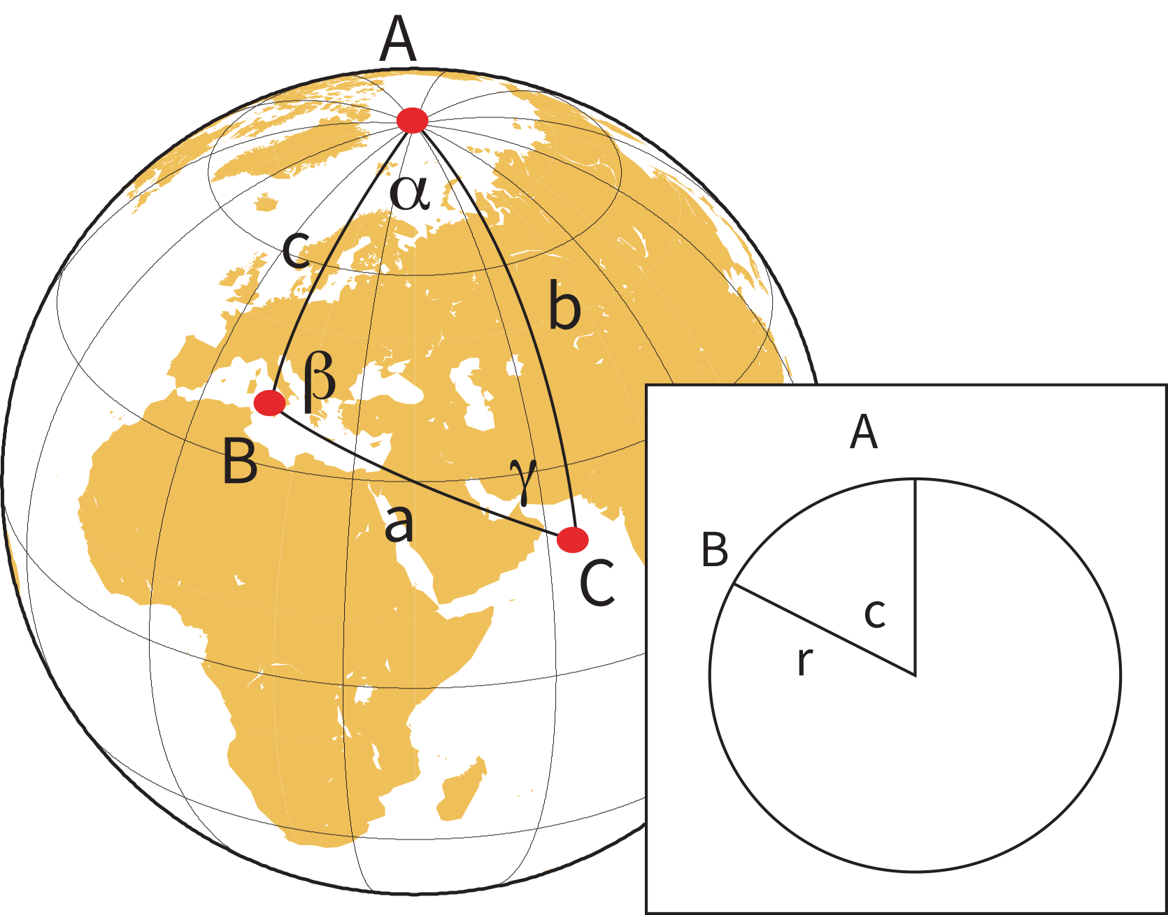
Figure A.1:Rules of spherical trigonometry. are all great circle tracks on a sphere which form a triangle with apices . The lengths of on a unit sphere are equal to the angles subtended by radii that intersect the globe at the apices, as shown in the inset. are the angles between the great circles.
In Figure A.1, and are the angles between the great circles labelled , , and . On a unit sphere, and are also the angles subtended by radii that intersect the globe at the apices A, B, and C (see inset on Figure A.1). Two formulae from spherical trigonometry come in handy in paleomagnetism, the Law of Sines:
and the Law of Cosines:
A.3.2Vector addition
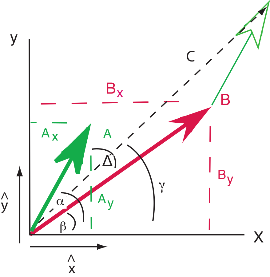
Figure A.2:Vectors and , their components A, B and the angles between them and the axis, and . The angle between the two vectors is . Unit vectors in the directions of the axes are and respectively.
To add the two vectors (see Figure A.2) and , we break each vector into components and . For example, where is the length of the vector . The components of the resultant vector are: . These can be converted back to polar coordinates of magnitude and angles if desired, whereby:
A.3.3Vector subtraction
To subtract two vectors, compute the components as in addition, but the components of the vector difference are: .
A.3.4Vector multiplication
There are two ways to multiply vectors. The first is the dot product whereby . This is a scalar and is actually the cosine of the angle between the two vectors if the and are taken as unit vectors (assume a magnitude of unity in the component calculation).
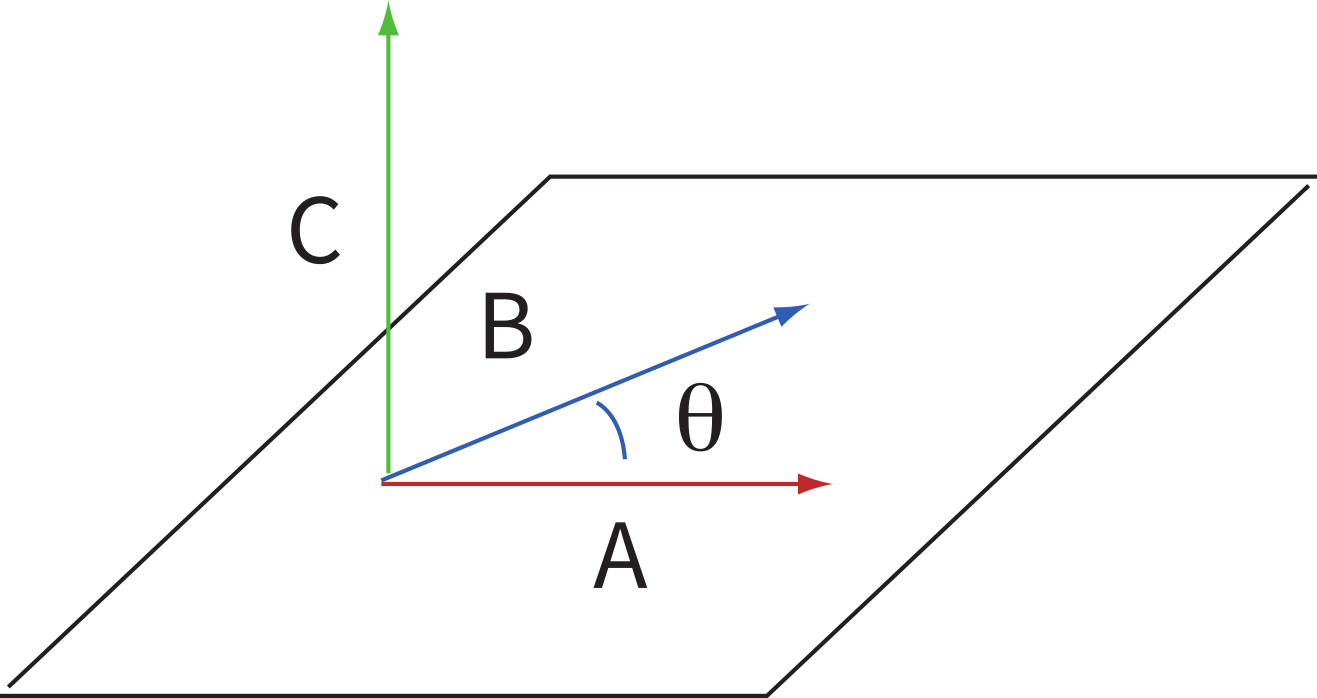
Figure A.3:Illustration of cross product of vectors and separated by angle to get the orthogonal vector .
The other way to perform vector multiplication is the cross product (see Figure A.3), which produces a vector orthogonal to both and and whose components are given by:
To calculate the determinant, we follow these rules:
or
A.3.5Tricks with tensors
Vectors belong to a more general concept called tensors. While a vector describes a magnitude of something in a given direction, tensors allow calculation of magnitudes as a function of orientation. Velocity is a vector relating speed to direction, but speed may change depending on direction, so we might need a tensor to calculate speed as a function of direction. Many properties in Earth science require tensors, like the indicatrix in mineralogy which relates the speed of light to crystallographic direction, or the relationship between stress and strain. Tensors in paleomagnetism are used, for example, to transform coordinate systems and to characterize the anisotropy of magnetic properties such as susceptibility. We will cover transformation of coordinate systems in the following.
A.3.5.1Direction cosines
We use direction cosines in paleomagnetism in a variety of applications, from mineralogy to transformation from specimen to geographic or stratigraphic coordinate systems. Direction cosines are the cosines of the angles between different axes in given coordinate systems, here and respectively (see, e.g., Figure A.4a). The direction cosine is the cosine of the angle between the and the , axes. We can define four of these direction cosines to fully describe the relationship between the two coordinate systems:
The first subscript always refers to the system and the second refers to the .
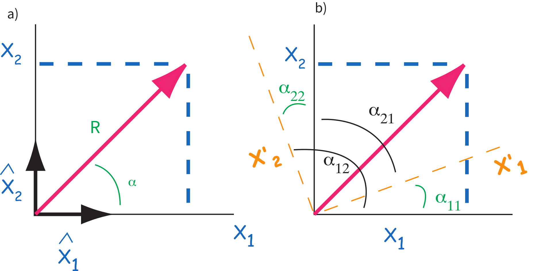
Figure A.4:Definition of direction cosines in two dimensions. a) Definition of vector in one set of coordinates, . b) Definition of angles relating axes to .
A.3.5.2Changing coordinate systems
One application of using direction cosines is the transformation of coordinates systems from one set () to a new set . To find new coordinates from the old (), we have:
In three dimensions we have:
which can also be written as:
with a short cut notation as: . However we write this, it means that for each axis , just sum through the ’s for all the dimensions. The matrix is an example of a 3 x 3 tensor and equations of the form relating two vectors with a tensor will be used throughout the book. A more common notation is with bold-faced variables which indicate vectors or tensors, e.g., .
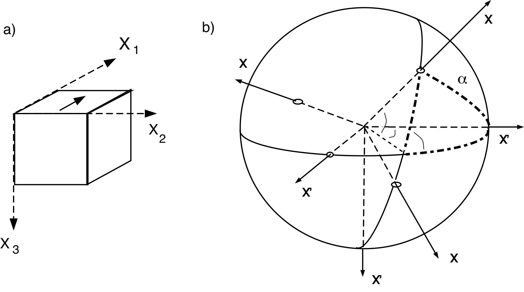
Figure A.5:a) Sample coordinate system. b) Trigonometric relations between two cartesian coordinate systems, and . are all known and the angles between the various axes can be calculated using spherical trigonometry. For example, the angle between and forms one side of the triangle shown by dash-dot lines. Thus, . [Figure from Tauxe (1998).]
Now we would like to apply this to changing coordinate systems for a paleomagnetic specimen in the most general case. The specimen coordinate system is defined by a right-hand rule where the thumb () is directed parallel to an arrow marked on the sample, the index finger () is in the same plane but at right angles and clockwise to and the middle finger () is perpendicular to the other two (Figure A.5a). The transformation of coordinates () from the axes to the coordinates in the desired coordinate system requires the determination of the direction cosines as described in Section A.3.5.1. The various can be calculated using spherical trigonometry as in Section A.3.1. For example, for the general case depicted in Figure A.5 is , which is given by the Law of Cosines (see Section A.3.1) by using appropriate values, or:
The other can be calculated in a similar manner. In the case of most coordinate system rotations used in paleomagnetism, is in the same plane as and (and is horizontal) so = 90°. This problem is much simpler. The directions cosines for the case where are:
The new coordinates can be obtained from Equation A.26, as follows:
The declination and inclination can be calculated by inserting these values in the equations in Chapter 2.
A.3.5.3Method for rotating points on a globe using finite rotation poles
Given the coordinates of the point on the globe with latitude , longitude the finite rotation pole with latitude , longitude , the way to transform coordinates is as follows (you should also review Section A.3.5.2).
Convert the latitudes and longitudes to cartesian coordinates by:
where is the point of interest.
Set up the rotation matrix as:
The coordinates of the transformed pole () are:
which can be converted back into latitude and longitude in the usual way (see Chapter 2).
A.3.5.4The orientation tensor and eigenvectors
The orientation tensor Scheidegger, 1965 (also known as the matrix of sums of squares and products), is extremely useful in paleomagnetism. This is found as follows:
Convert the , , and for a set of data points (e.g., a sequence of demagnetization data, or a set of geomagnetic vectors or unit vectors where ) to corresponding values (see Chapter 2).
Calculate the coordinates of the “center of mass” () of the data points:
where is the number of data points involved. Note that for unit vectors, the center of mass is the same as the Fisher mean (Chapter 11).
Transform the origin of the data cluster to the center of mass:
where are the transformed coordinates.
The orientation matrix is defined as:
is a 3 x 3 matrix, where only six of the nine elements are independent. It is constructed in some coordinate system, such as the geographic or sample coordinate system. Usually, none of the six independent elements are zero. There exists, however, a coordinate system along which the “off-axis” terms are zero and the axes of this coordinate system are called the eigenvectors of the matrix. The three elements of in the eigenvector coordinate system are called eigenvalues. In terms of linear algebra, this idea can be expressed as:
where is the matrix containing three eigenvectors and is the diagonal matrix containing three eigenvalues. Equation A.48 is only true if:
If we expand Equation A.49, we have a third degree polynomial whose roots () are the eigenvalues:
The three possible values of () can be found with iteration and determination. In practice, there are many programs for calculating . My personal favorite is the Numpy Module for Python (see many free websites, especially Scientific Python (SciPy) for hints). Please note that the conventions adopted here are to scale the ’s such that they sum to one; the largest eigenvalue is termed and corresponds to the eigenvector .
Inserting the values for the transformed components calculated in Equation A.46 into gives the covariance matrix for the demagnetization data. The direction of the axis associated with the greatest scatter in the data (the principal eigenvector ) corresponds to a best-fit line through the data. This is usually taken to be the direction of the component in question. This direction also corresponds to the axis around which the “moment of inertia” is least. The eigenvalues of are the variances associated with each eigenvector. Thus the standard deviations are .
A.3.6Upside down triangles, 
A.3.6.1Gradient
We often wish to differentiate a function along three orthogonal axes. For example, imagine we know the topography of a ski area (see Figure A.6). For every location (in say, and coordinates), we know the height above sea level. This is a scalar function. Now imagine we want to build a ski resort, so we need to know the direction of steepest descent and the slope (red arrows in Figure A.6).
Figure A.6:Illustration of the relationship between a vector field (direction and magnitude of steepest slope at every point, e.g., red arrows) and the scalar field (height) of a ski slope.
To convert the scalar field (height versus position) to a vector field (direction and magnitude of greatest slope) mathematically, we would simply differentiate the topography function. Let’s say we had a very weird two dimensional, sinusoidal topography such that with the height and is the distance from some marker. The slope in the direction (), then would be . If were a three dimensional topography then the gradient of the topography function would be:
For short hand, we define a “vector differential operator” to be a vector whose components are
This can also be written in polar coordinates:
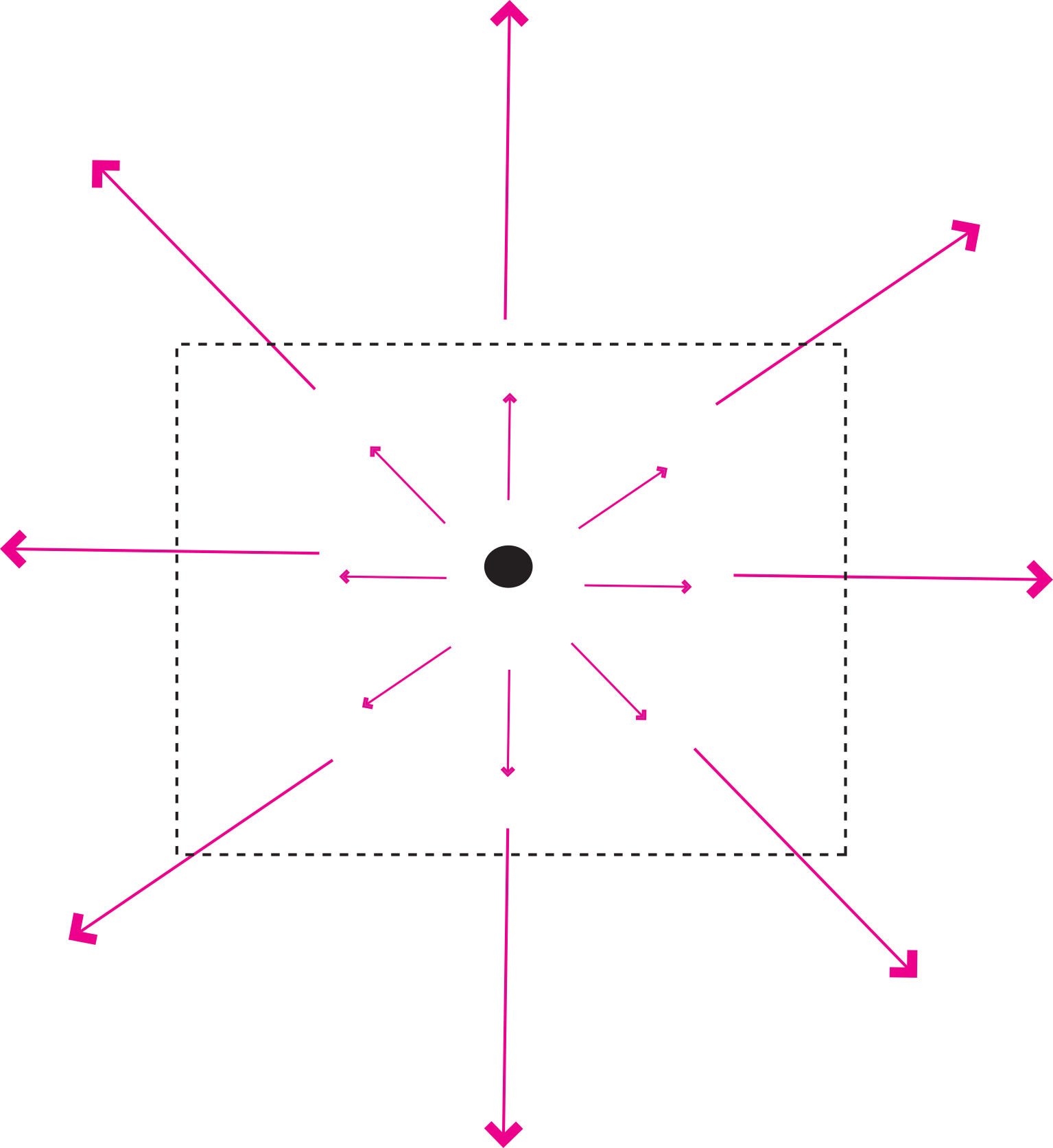
Figure A.7:Example of a vector field with a non-zero divergence.
A.3.6.2Divergence
The divergence of a vector function (e.g. ) is written as:
The trick here is to treat as a vector and use the rules for dot products described in Section A.3.2. In cartesian coordinates, this is:
Like all dot products, the divergence of a vector function is a scalar.
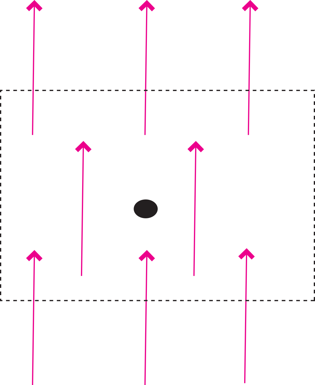
Figure A.8:Example of a vector field with zero divergence.
Figure A.9:Example of a vector field with non-zero curl.
The name divergence is well chosen because is a measure of how much the vector field “spreads out” (diverges) from the point in question. In fact, what divergence quantifies is the balance between vectors coming in to a particular region versus those that go out. The example in Figure A.7 depicts a vector function whereby the magnitude of the vector increases linearly with distance away from the central point. An example of such a function would be . The divergence of this function is:
(a scalar). There are no arrows returning in to the dashed box, only vectors going out and the non-zero divergence quantifies this net flux out of the box.
Now consider Figure A.8, which depicts a vector function that is constant over space, i.e. . The divergence of this function is:
The zero divergence means that for every vector leaving the box, there is an equal and opposite vector coming in. Put another way, no net flux results in a zero divergence. The fact that the divergence of the magnetic field is zero means that there are no point sources (monopoles), as opposed to electrical fields that have divergence related to the presence of electrons or protons.
A.3.6.3Curl
The curl of the vector function is defined as . In cartesian coordinates we have
Curl is a measure of how much the vector function “curls” around a given point. The function describing the velocity of water in a whirlpool has a significant curl, while that of a smoothly flowing stream does not.
Consider Figure A.9 which depicts a vector function . The curl of this function is:
or
So there is a positive curl in this function and the curl is a vector in the direction.
The magnetic field has a non-zero curl in the presence of currents or changing electric fields. In free space, away from currents (lightning!!), the magnetic field has zero curl.
A.3.7The statistical bootstrap
Sometimes things just are not normal. Statistically that is. When you can not assume that your data follow some known distribution, like the normal distribution, or the Fisher distribution, what do you do? In this section, we outline a technique called the bootstrap, which allows us to make statistical inferences when parametric assumptions fail. The reader should also refer to Efron & Tibshirani (1993) for a more complete discussion.
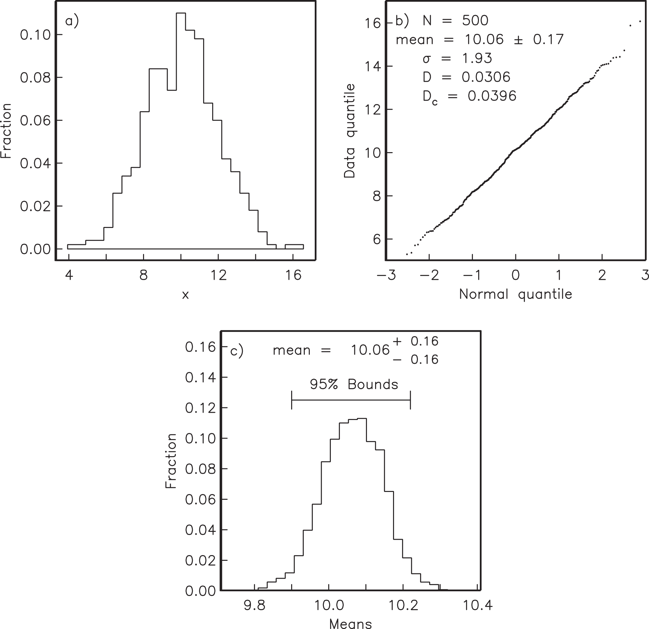
Figure A.10:Bootstrapping applied to a normal distribution. a) 500 data points are drawn from a Gaussian distribution with mean of 10 and a standard deviation of 2. b) Q-Q plot of data in a). The 95% confidence interval for the mean is given by Gauss statistics as ± 0.17. 10,000 new (para) data sets are generated by randomly drawing data points from the original data set shown in a). c) A histogram of the means from all the para-data sets. 95% of the means fall within the interval 10.06, hence the bootstrap confidence interval is similar to that calculated with Gaussian statistics. [Figure from Tauxe (1998).]
In Figure A.10, we illustrate the essentials of the statistical bootstrap. We will develop the technique using data drawn from a normal distribution. First, we generate a synthetic data set by drawing 500 data points from a normal distribution with a mean of 10 and a standard deviation of 2. The synthetic data are plotted as a histogram in Figure A.10a. In Figure A.10b we plot the data as a Q-Q plot (see Section B.1.5) against the expected for a normal distribution.
The data in Figure A.10a plot in a line on the Q-Q plot (Figure A.10b). The value for is 0.0306. Because , the critical value of , at the 95% confidence level is 0.0396. Happily, our normal distribution simulation program has produced a set of 500 numbers for which the null hypothesis of a normal distribution has not been rejected. The mean of the synthetic dataset is about 10 and the standard deviation is 1.9. The usual Gaussian statistics allow us to estimate a 95% confidence interval for the mean as or .
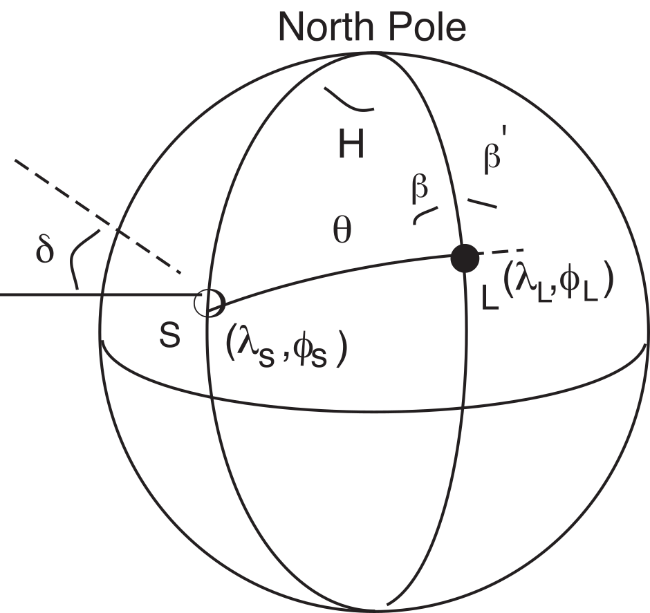
Figure A.11:Calculation of the azimuth of the shadow direction () relative to true North, using a sun compass. L is the site location (at ), S is the position on the Earth where the sun is directly overhead (). [Figure from Tauxe (1998).]
In order to estimate a confidence interval for the mean using the bootstrap, we first randomly draw a list of data by selecting data points from the original data set. This list is called a pseudo-sample of the data. Some data points will be used more than once and others will not be used at all. We then calculate the mean of the pseudo-sample. We repeat the procedure of drawing pseudo-samples and calculating the mean many times (say 10,000 times). A histogram of the “bootstrapped” means is plotted in Figure A.10c. If these are sorted such that the first mean is the lowest and the last mean is the highest, the 95% of the means are between the 250 and the 9,750 mean. These therefore are the 95% confidence bounds because we are approximately 95% confident that the true mean lies between these limits. The 95% confidence interval calculated for the data in Figure A.10 by bootstrap is about ± 0.16 which is nearly the same as that calculated the Gaussian way. However, the bootstrap required orders of magnitude more calculations than the Gaussian method, hence it is ill-advised to perform a bootstrap calculation when a parametric one will do. Nonetheless, if the data are not Gaussian, the bootstrap provides a means of calculating confidence intervals when there is no quick and easy way. Furthermore, with a modern computer, the time required to calculate the bootstrap illustrated in Figure A.10 was virtually imperceptible.
A.3.8Directions using a sun compass
In a sun compass problem, we have the direction of the sun’s shadow and an angle between that and the desired direction (). The declination of the shadow itself is 180° from the direction toward the sun. In Figure A.11, the problem of calculating declination from sun compass information is set up as a spherical trigonometry problem, similar to those introduced in Chapter 2 and Section A.3.1. The declination of the shadow direction , is given by 180 - . We also know the latitude of the sampling location L (). We need to calculate the latitude of S (the point on the Earth’s surface where the sun is directly overhead), and the local hour angle .
Knowing the time of observation (in Universal Time), the position of S ( in Figure A.11) can be calculated with reasonable precision (to within 0.01°) for the period of time between 1950 and 2050 using the procedure recommended in the 1996 Astronomical Almanac:
First, calculate the Julian Day . Then, calculate the fraction of the day in Universal Time . Finally, calculate the parameter which is the number of days from J2000 by:
The mean longitude of the sun (), corrected for aberration, can be estimated in degrees by:
The mean anomaly (in degrees).
Put and in the range 0 → 360°.
The longitude of the ecliptic is given by (in degrees).
The obliquity of the ecliptic is given by .
Calculate the right ascension () by:
where and tan.
The so-called “declination” of the sun ( in Figure A.11 which should not be confused with the magnetic declination ), which we will use as the latitude , is given by:
Finally, the equation of time in degrees is given by .
We can now calculate the Greenwich Hour Angle from the Universal Time (in minutes) by . The local hour angle ( in Figure A.11) is . We calculate using the laws of spherical trigonometry (see Section A.3.1). First we calculate by the Law of Cosines (remembering that the cosine of the colatitude equals the sine of the latitude):
and finally using the Law of Sines:
If , then the required angle is the shadow direction , given by: . The azimuth of the desired direction is plus the measured shadow angle .
- Tauxe, L. (1998). Paleomagnetic Principles and Practice. Kluwer Academic Publishers.
- Scheidegger, A. E. (1965). On the statistics of the orientation of bedding planes, grain axes, and similar sedimentological data. U.S. Geological Survey Professional Paper, 525–C, 164–167.
- Efron, B., & Tibshirani, R. J. (1993). An Introduction to the Bootstrap (Vol. 57). Chapman. 10.1201/9780429246593