One of the major efforts in paleomagnetism has been to study ancient geomagnetic fields. Because human measurements extend back about a millennium, measurement of “accidental” records provided by archaeological or geological materials remains the only way to investigate ancient field behavior. Therefore it is useful for students of paleomagnetism to understand something about the present geomagnetic field. In this chapter we review the general properties of the Earth’s magnetic field.
The part of the geomagnetic field of interest to paleomagnetists is generated by convection currents in the liquid outer core of the Earth which is composed of iron, nickel and some unknown lighter component(s). The source of energy for this convection is not known for certain, but is thought to be partly from cooling of the core and partly from the buoyancy of the iron/nickel liquid outer core caused by freezing out of the pure iron inner core. Motions of this conducting fluid are controlled by the buoyancy of the liquid, the spin of the Earth about its axis and by the interaction of the conducting fluid with the magnetic field (in a horribly non-linear fashion). Solving the equations for the fluid motions and resulting magnetic fields is a challenging computational task. Recent numerical models, however, show that such magnetohydrodynamical systems can produce self-sustaining dynamos which create enormous external magnetic fields.
2.1Components of magnetic vectors
The magnetic field of a dipole aligned along the spin axis and centered in the Earth (a so-called geocentric axial dipole, or GAD) is shown in Figure 2.1a. [See Chapter 1 for a derivation of how to find the radial and tangential components of such a field.] By convention, the sign of the Earth’s dipole is negative, pointing toward the south pole as shown in Figure 2.1a and magnetic field lines point toward the north pole. They point downward in the northern hemisphere and upward in the southern hemisphere.
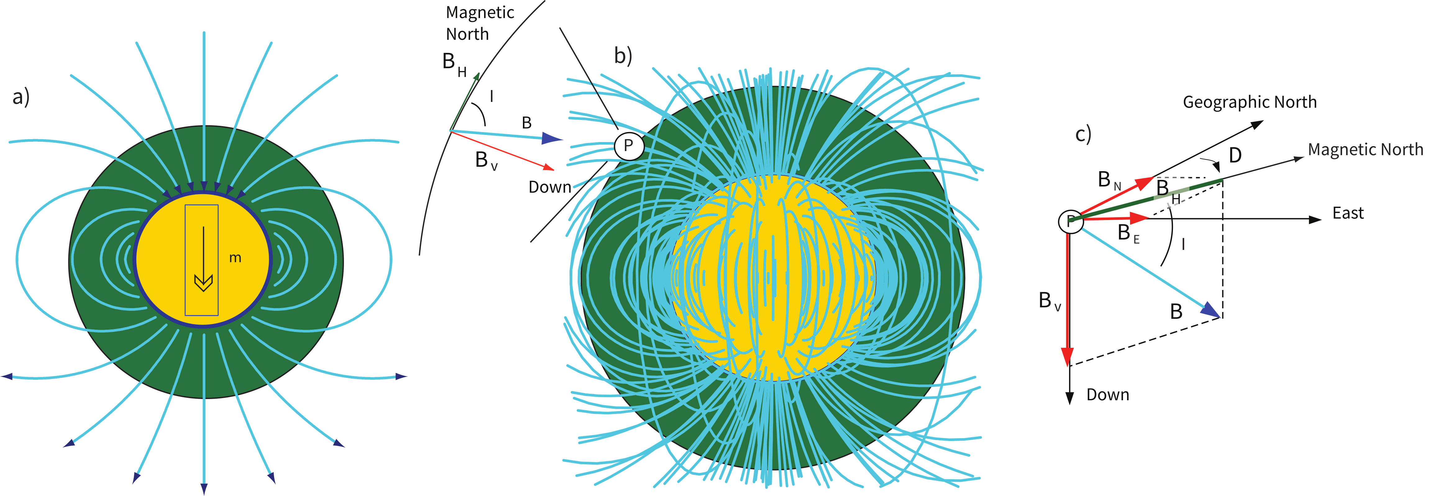
Figure 2.1:a) Lines of flux produced by a geocentric axial dipole. b) Lines of flux of the geomagnetic field of 2005. At point P the horizontal component of the field , is directed toward the magnetic north. The vertical component is directed down and the field makes an angle with the horizontal, known as the inclination. c) Components of the geomagnetic field vector . The angle between the horizontal component (directed toward magnetic north and geographic north is the declination .) [Modified from Ben-Yosef et al. (2008).]
Although dominantly dipolar, the geomagnetic field is not perfectly modeled by a geocentric axial dipole, but is somewhat more complicated (see Figure 2.1b). At the point on the surface labeled ‘P’, the geomagnetic field points nearly north and down at an angle of approximately 60°. Vectors in three dimensions are described by three numbers and in many paleomagnetic applications, these are two angles ( and ) and the strength () as shown in Figure 2.1b and c. The angle from the horizontal plane is the inclination ; it is positive downward and ranges from +90° for straight down to -90° for straight up. If the geomagnetic field were that of a perfect GAD field, the horizontal component of the magnetic field ( in Figure 2.1b) would point directly toward geographic north. In most places on the Earth there is a deflection away from geographic north and the angle between geographic and magnetic north is the declination, (see Figure 2.1c). is measured positive clockwise from North and ranges from . [Westward declinations can also be expressed as negative numbers, i.e., 350° = -10°.] The vertical component ( in Figure 2.1b,c) of the geomagnetic field at P, is given by
and the horizontal component (Figure 2.1c) by
can be further resolved into north and east components ( and in Figure 2.1c) by
Depending on the particular problem, some coordinate systems are more suitable to use because they have the symmetry of the problem built into them. We have just defined a coordinate system using two angles and a length () and the equivalent Cartesian coordinates of (). We will need to convert among them at will. There are many names for the Cartesian coordinates. In addition to north, east and down, they could also be or even and . The convention used in this book is that axes are denoted , while the components along the axes are frequently designated . In the geographic frame of reference, positive is to the north, is east and is vertically down in keeping with the right-hand rule. To convert from Cartesian coordinates to angular coordinates ():
Be careful of the sign ambiguity of the tangent function. You may well end up in the wrong quadrant and have to add 180°; this will happen if both and are negative. In most computer languages, there is a function atan2 which takes care of this, but most hand calculators will not. Remember that most computer languages expect angles to be given in radians, not degrees, so multiply degrees by to convert to radians. Note also that in place of for magnetic induction with units of tesla as a measure of vector length, (see Chapter 1), we could also use , (both Am) or (Am) for magnetic field, magnetization or magnetic moment respectively.
2.2Reference magnetic field
We can measure declination, inclination and intensity at different places around the globe, but not everywhere all the time. Yet it is often handy to be able to predict what these components are. For example, it is extremely useful to know what the deviation is between true North and declination in order to find our way with maps and compasses. In principle, magnetic field vectors can be derived from the magnetic potential as we showed in Chapter 1. For an axial dipolar field, there is but one scalar coefficient (the magnetic moment of a dipole source). For the geomagnetic field, there are many more coefficients, including not just an axial dipole aligned with the spin axis, but two orthogonal equatorial dipoles and a whole host of more complicated sources such as quadrupoles, octupoles and so on. A list of coefficients associated with these sources allows us to calculate the magnetic field vector anywhere outside of the source region. In this section, we outline how this might be done.
As we learned in Chapter 1, the magnetic field at the Earth’s surface can be calculated from the gradient of a scalar potential field (), and this scalar potential field satisfies Laplace’s Equation:
For the geomagnetic field (ignoring external sources of the magnetic field which are in any case small and transient), the potential equation can be written as:
where is the radius of the Earth ( m). In addition to the radial distance and the angle away from the pole , there is , the angle around the equator from some reference, say, the Greenwich meridian. Here, is the co-latitude and is the longitude. The s and s are the Gauss coefficients (degree and order ) for hypothetical sources at radii less than calculated for a particular year. These are normally given in units of nT. The s are wiggly functions called partially normalized Schmidt polynomials of the argument . These are closely related to the associated Legendre polynomials. [When the Schmidt and Legendre polynomials are identical.] The first few s are:
and are shown in Figure 2.2.
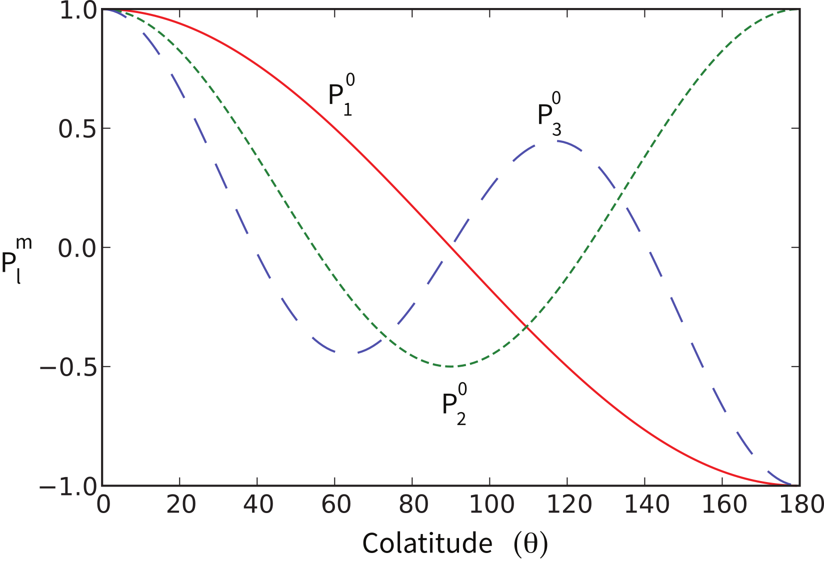
Figure 2.2:Schmidt polynomials.
To get an idea of how the Gauss coefficients in the potential relate to the associated magnetic fields, we show three examples in Figure 2.3. We plot the inclinations of the vector fields that would be produced by the terms with and respectively. These are the axial () dipole (), quadrupole () and octupole () terms. The associated potentials for each harmonic are shown in the insets.
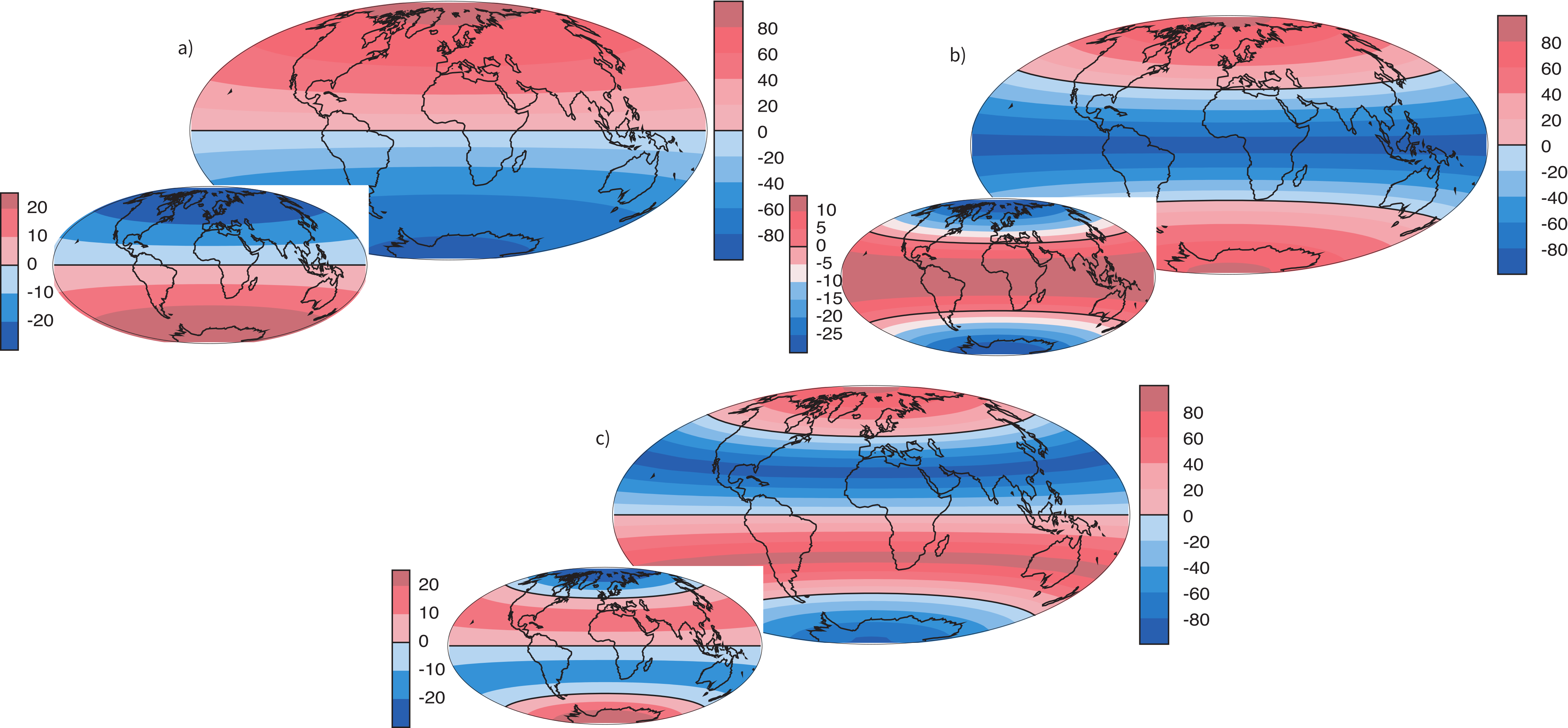
Figure 2.3:Examples of potential fields (insets) and maps of the associated patterns for global inclinations. Each coefficient is set to 30 T. a) Dipole (T), b) Quadrupole (T), c) Octupole (T).
In general, terms for which the difference between the subscript () and the superscript () is odd (e.g., the axial dipole and octupole ) produce magnetic fields that are antisymmetric about the equator, while those for which the difference is even (e.g., the axial quadrupole ) have symmetric fields. In Figure 2.3a we show the inclinations produced by a purely dipolar field of the same sign as the present day field. The inclinations are all positive (down) in the northern hemisphere and negative (up) in the southern hemisphere. In contrast, inclinations produced by a purely quadrupolar field (Figure 2.3b) are down at the poles and up at the equator. The map of inclinations produced by a purely axial octupolar field (Figure 2.3c) are again asymmetric about the equator with vertical directions of opposite signs at the poles separated by bands with the opposite sign at mid-latitudes.
As noted before, there is not one, but three dipole terms in Equation 2.6, the axial term () and two equatorial terms ( and ). Therefore, the total dipole contribution is the vector sum of these three or . The total quadrupole contribution () combines five coefficients and the total octupole () contribution combines seven coefficients.
So how do we get this marvelous list of Gauss coefficients? If you want to know the details, please refer to Langel (1987). We will just give a brief introduction here. Recalling Chapter 1, once the scalar potential is known, the components of the magnetic field can be calculated from it. We solved this for the radial and tangential field components ( and ) in Chapter 1. We will now change coordinate and unit systems and introduce a third dimension (because the field is not perfectly dipolar). The north, east, and vertically down components are related to the potential by:
where , , are radius, co-latitude (degrees away from the North pole) and longitude, respectively. Here, is positive down, is positive east, and is positive to the north, the opposite of and as defined in Chapter 1. Note that Equation 2.8 is in units of induction, not Am if the units for the Gauss coefficients are in nT, as is the current practice.
Going backwards, the Gauss coefficients are determined by fitting Equations 2.8 and 2.6 to observations of the magnetic field made by magnetic observatories or satellite for a particular time. The International (or Definitive) Geomagnetic Reference Field or I(D)GRF, for a given time interval is an agreed upon set of values for a number of Gauss coefficients and their time derivatives. IGRF (or DGRF) models and programs for calculating various components of the magnetic field are available on the internet from the National Geophysical Data Center; the address is http://
In practice, the Gauss coefficients for a particular reference field are estimated by least-squares fitting of observations of the geomagnetic field. You need a minimum of 48 observations to estimate the coefficients to . Nowadays, we have satellites which give us thousands of measurements and the list of generation 10 of the IGRF for 2005 goes to .
Table 2.1:IGRF, 12th generation (2015) to Thébault et al., 2015.
| (nT) | (nT) | (nT) | (nT) | ||||
|---|---|---|---|---|---|---|---|
| 1 | 0 | -29442.0 | 0 | 5 | 0 | -232.6 | 0 |
| 1 | 1 | -1501.0 | 4797.1 | 5 | 1 | 360.1 | 47.3 |
| 2 | 0 | -2445.1 | 0 | 5 | 2 | 192.4 | 197.0 |
| 2 | 1 | 3012.9 | -2845.6 | 5 | 3 | -140.9 | -119.3 |
| 2 | 2 | 1676.7 | -641.9 | 5 | 4 | -157.5 | 16.0 |
| 3 | 0 | 1350.7 | 0 | 5 | 5 | 4.1 | 100.2 |
| 3 | 1 | -2352.3 | -115.3 | 6 | 0 | 70.0 | 0 |
| 3 | 2 | 1225.6 | 244.9 | 6 | 1 | 67.7 | -20.8 |
| 3 | 3 | 582.0 | -538.4 | 6 | 2 | 72.7 | 33.2 |
| 4 | 0 | 907.6 | 0 | 6 | 3 | -129.9 | 58.9 |
| 4 | 1 | 813.7 | 283.3 | 6 | 4 | -28.9 | -66.7 |
| 4 | 2 | 120.4 | -188.7 | 6 | 5 | 13.2 | 7.3 |
| 4 | 3 | -334.9 | 180.9 | 6 | 6 | -70.9 | 62.6 |
| 4 | 4 | 70.4 | -329.5 |
In order to get a feel for the importance of the various Gauss coefficients, take a look at Table 2.1, which has the Schmidt quasi-normalized Gauss coefficients for the first six degrees from the IGRF for 2005. The power at each degree is the average squared field per spherical harmonic degree over the Earth’s surface and is calculated by Lowes, 1974. The so-called Lowes spectrum is shown in Figure 2.4. It is clear that the lowest order terms (degree one) totally dominate, constituting some 90% of the field. This is why the geomagnetic field is often assumed to be equivalent to a magnetic field created by a simple dipole at the center of the Earth.
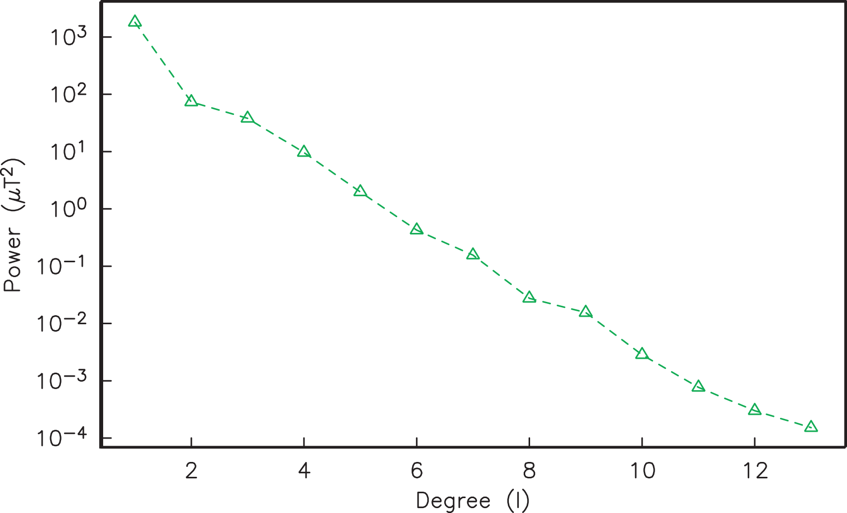
Figure 2.4:Power at the Earth’s surface of the geomagnetic field versus degree for the 2005 IGRF (Table 2.1).
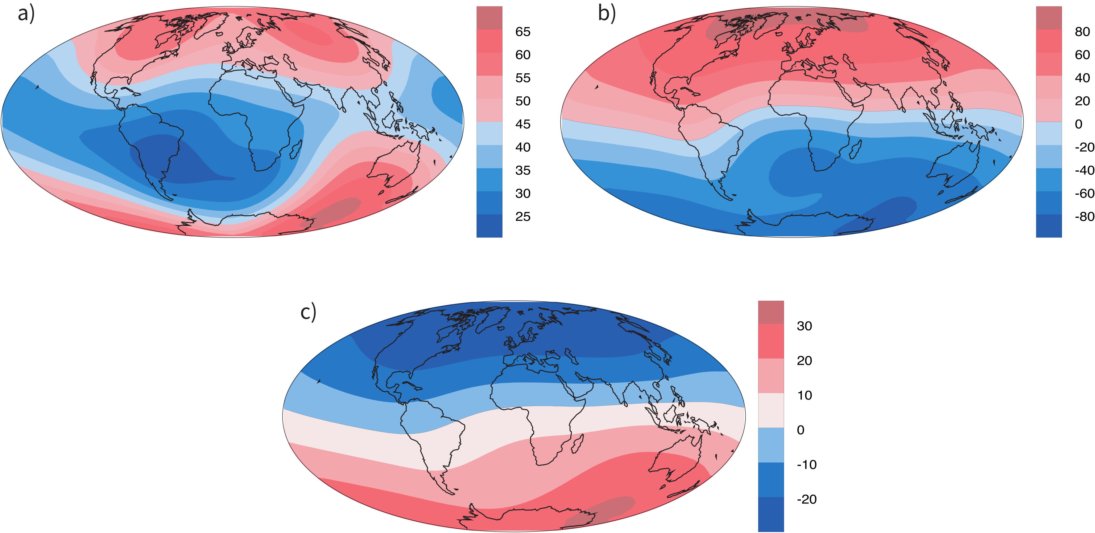
Figure 2.5:Maps of geomagnetic field of the IGRF for 2005. a) Intensity (units of T), b) inclination, c) potential (units of nT).
2.3Geocentric axial dipole (GAD) and other poles
The beauty of using the geomagnetic potential field is that the vector field can be evaluated anywhere outside the source region. Using the values for a given reference field in Equations 2.6 and 2.8, we can calculate values of and at any location on Earth. Figure 2.1b shows the lines of flux predicted from the 2005 IGRF from the core-mantle boundary up. We can see that the field becomes simpler and more dipolar as we move from the core mantle boundary to the surface. Yet, there is still significant non-dipolar structure in the geomagnetic field even at the Earth’s surface.
We can recast the vectors at the surface of the Earth into maps of components as shown in Figure 2.5a,b. We show the potential in Figure 2.5c for comparison with that of a pure dipole (inset to Figure 2.3a). These maps illustrate the fact that the field is a complicated function of position on the surface of the Earth. The intensity values in Figure 2.5a are, in general, highest near the poles (~60 T) and lowest near the equator (~30 T), but the contours are not straight lines parallel to latitude as they would be for a field generated strictly by a geocentric axial dipole (GAD) (e.g, Figure 2.1a). Similarly, a GAD would produce lines of inclination that vary in a regular way from -90° to +90° at the poles, with 0° at the equator; the contours would parallel the lines of latitude. Although the general trend in inclination shown in Figure 2.5b is similar to the GAD model, the field lines are more complicated, which again suggests that the field is not perfectly described by a geocentric bar magnet.
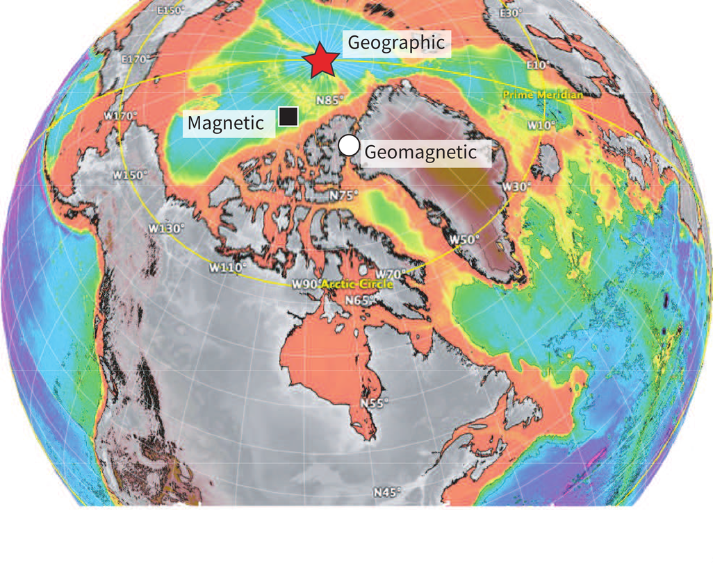
Figure 2.6:Different poles. The square is the magnetic North Pole, where the magnetic field is straight down (82.7°N, 114.4°W for the IGRF 2005); the circle is the geomagnetic North Pole, where the axis of the best fitting dipole pierces the surface (9.7°N, 71.8°W for the IGRF 2005). The star is the geographic North Pole. [Figure made using Google Earth with seafloor topography of D. Sandwell supplied to Google Earth by D. Staudigel.]
Perhaps the most important result of spherical harmonic analysis for our purposes is that the field at the Earth’s surface is dominated by the degree one terms () and the external contributions are very small. The first order terms can be thought of as geocentric dipoles that are aligned with three different axes: the spin axis () and two equatorial axes that intersect the equator at the Greenwich meridian () and at 90° East (). The vector sum of these geocentric dipoles is a dipole that is currently inclined by about 10° to the spin axis. The axis of this best-fitting dipole pierces the surface of the Earth at the circle in Figure 2.6. This point and its antipode are called geomagnetic poles. Points at which the field is vertical ( shown by a square in Figure 2.6) are called magnetic poles, or sometimes dip poles. These poles are distinguishable from the geographic poles, where the spin axis of the Earth intersects its surface. The northern geographic pole is shown by a star in Figure 2.6.
It turns out that when averaged over sufficient time, the geomagnetic field actually does seem to be approximately a GAD field, perhaps with a pinch of thrown in (see e.g., Merrill et al. (1996)). The GAD model of the field will serve as a useful crutch throughout our discussions of paleomagnetic data and applications. Averaging ancient magnetic poles over enough time to average out secular variation (thought to be 10 or 10 years) gives what is known as a paleomagnetic pole; this is usually assumed to be co-axial with the Earth’s geographic pole (the spin axis).
Because the geomagnetic field is axially dipolar to a first approximation, we can write:
Note that is given in nT in Table 2.1. Thus, from Equation 2.9,
Given some latitude on the surface of the Earth in Figure 2.1a and using the equations for and , we find that:
This equation is sometimes called the dipole formula and shows that the inclination of the magnetic field is directly related to the co-latitude () for a field produced by a geocentric axial dipole (or ). The dipole formula allows us to calculate the latitude of the measuring position from the inclination of the (GAD) magnetic field, a result that is fundamental in plate tectonic reconstructions. The intensity of a dipolar magnetic field is also related to (co)latitude because:
The dipole field intensity has changed by more than an order of magnitude in the past and the dipole relationship of intensity to latitude turns out to be not useful for tectonic reconstructions.
2.4Plotting magnetic directional data
Magnetic field and magnetization directions can be visualized as unit vectors anchored at the center of a unit sphere. Such a unit sphere is difficult to represent on a 2-D page. There are several popular projections, including the Lambert equal area projection which we will be making extensive use of in later chapters. The principles of construction of the equal area projection are covered in Section B.1.
In general, regions of equal area on the sphere project as equal area regions on this projection, as the name implies. Plotting directional data in this way enables rapid assessment of data scatter. A drawback of this projection is that circles on the surface of a sphere project as ellipses. Also, because we have projected a vector onto a unit sphere, we have lost information concerning the magnitude of the vector. Finally, lower and upper hemisphere projections must be distinguished with different symbols. The paleomagnetic convention is: lower hemisphere projections (downward directions) use solid symbols, while upper hemisphere projections are open.
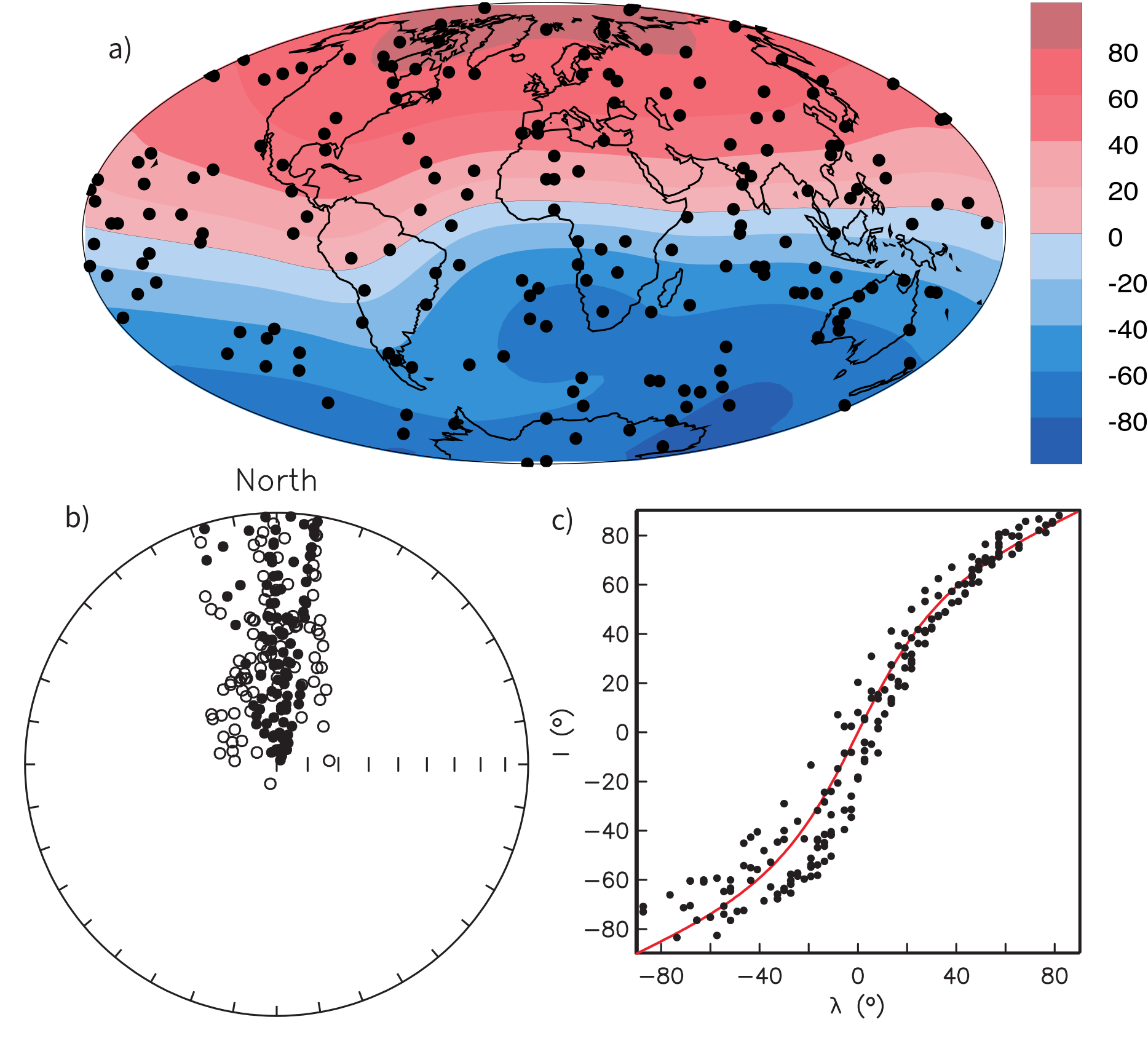
Figure 2.7:a) Hammer projection of 200 randomly selected locations around the globe. b) Equal area projection of directions of Earth’s magnetic field as given by the IGRF evaluated for the year 2005 at locations shown in a). Open (closed) symbols indicate upper (lower) hemisphere. c) Inclinations (I) plotted as a function of site latitude (). The solid line is the inclination expected from the dipole formula (see text). Negative latitudes are south and negative inclinations are up. [Figure redrawn from Tauxe (1998).]
The dipole formula allows us to convert a given measurement of to an equivalent magnetic co-latitude :
If the field were a simple GAD field, would be a reasonable estimate of , but non-GAD terms can invalidate this assumption. To get a feel for the effect of these non-GAD terms, we consider first what would happen if we took random measurements of the Earth’s present field (see Figure 2.7). We evaluated the directions of the magnetic field using the IGRF for 2005 at 200 positions on the globe (shown in Figure 2.7a). These directions are plotted in Figure 2.7b using the paleomagnetic convention of open symbols pointing up and closed symbols pointing down. In Figure 2.7c, we plot the inclinations as a function of latitude. As expected from a predominantly dipolar field, inclinations cluster around the values for a geocentric axial dipolar field but there is considerable scatter and interestingly the scatter is larger in the southern hemisphere than in the northern one. This is related to the low intensities beneath South America and the Atlantic region seen in Figure 2.5a.
2.4.1 transformation
Often we wish to compare directions from distant parts of the globe. There is an inherent difficulty in doing so because of the large variability in inclination with latitude. In such cases it is appropriate to consider the data relative to the expected direction (from GAD) at each sampling site. For this purpose, it is useful to use a transformation whereby each direction is rotated such that the direction expected from a geocentric axial dipole field (GAD) at the sampling site is the center of the equal area projection. This is accomplished as follows:
Each direction is converted to Cartesian coordinates () by:
These are rotated to the new coordinate system (, see Section A.3.5.2) by:
where = the inclination expected from a GAD field (), is the site latitude, and is the inclination of the paleofield vector projected onto the N-S plane (). The are then converted to by Equation 2.4.
In Figure 2.8a we show the geomagnetic field vectors evaluated at random longitudes along a latitude band of 45°N. The vectors are shown in their Cartesian coordinates of North, East and Down. In Figure 2.8b we show what happens when we rotate the coordinate system to peer down the direction expected from an axial dipolar field at 45°N (which has an inclination of 63°). The vectors circle about the expected direction. Finally, we see what happens to the directions shown in Figure 2.7b after the transformation in Figure 2.8. These are unit vectors projected along the expected direction for each observation in Figure 2.7a. Comparing the equal area projection of the directions themselves (Figure 2.7b) to the transformed directions (Figure 2.8c), we see that the latitudinal dependence of the inclinations has been removed.
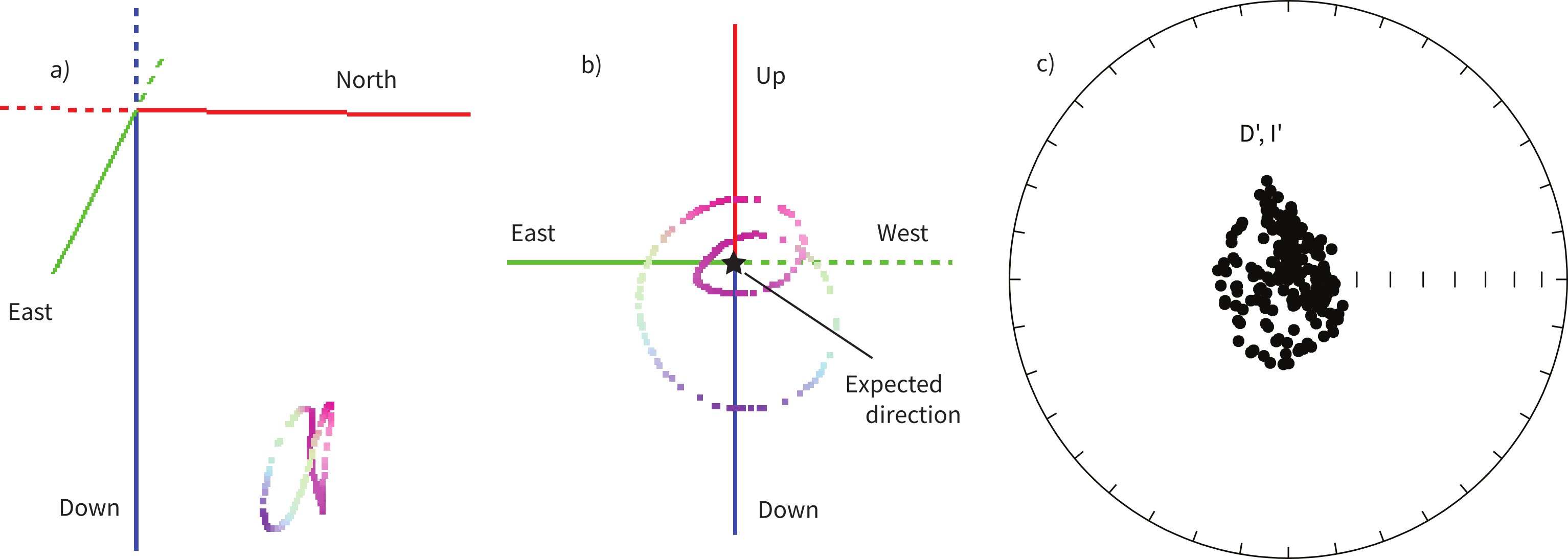
Figure 2.8:a) Vectors evaluated around the globe at 45°N. Red/green/blue colors reflect the North, East and Down components respectively. b) The unit vectors (assuming unit length) from a). c) Directions from Figure 2.7b transformed using the transformation.
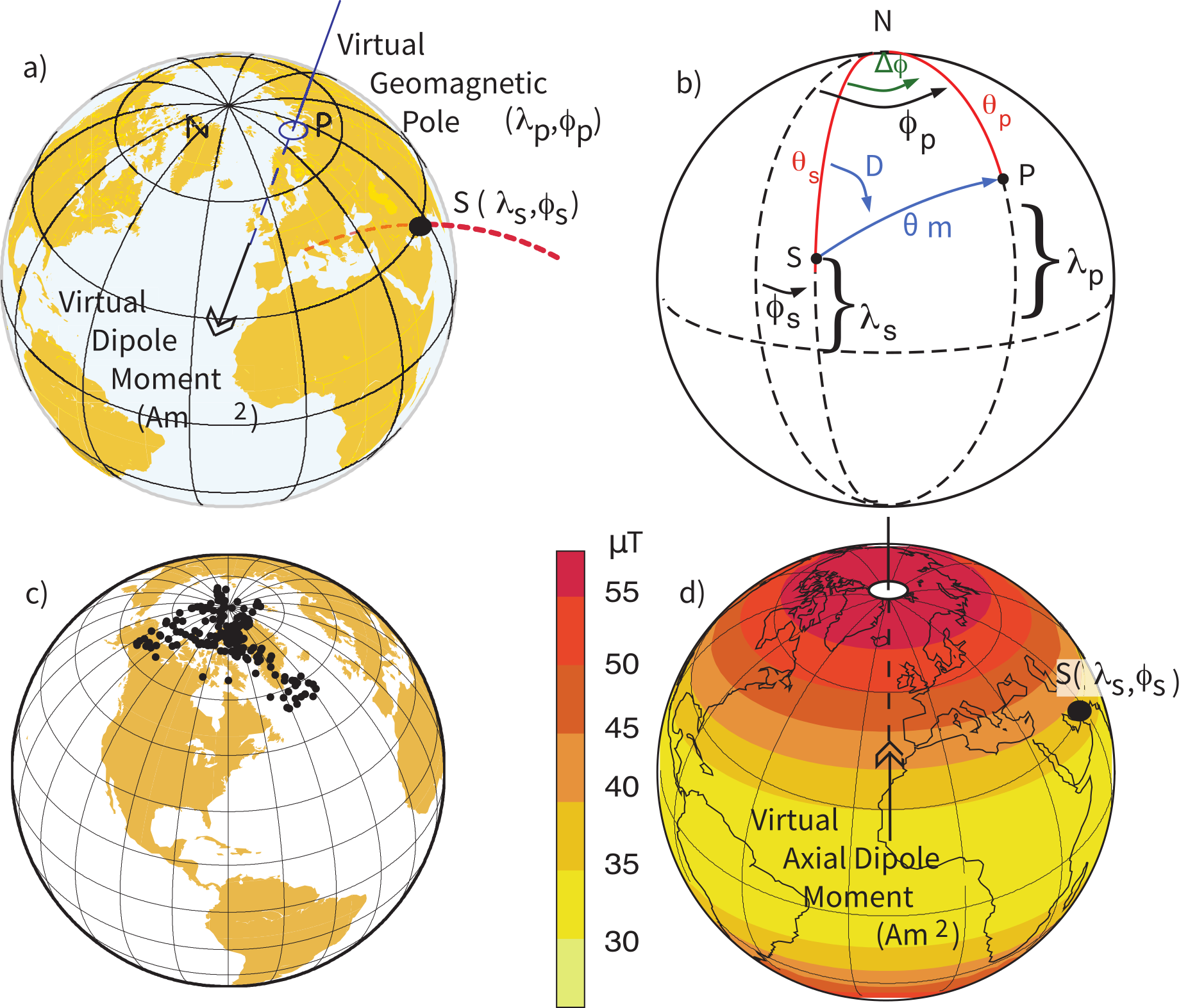
Figure 2.9:Transformation of a vector measured at S into a virtual geomagnetic pole position (VGP) and virtual dipole moment (VDM), using principles of spherical trigonometry and the dipole formula. a) Red dashed line is the magnetic field line observed at S (latitude of , longitude of ). This field line is the same as one produced by the VDM at the center of the Earth. The point where the axis of the VDM pierces the Earth’s surface is the VGP. b) Observed declination (D) and inclination (converted to using the dipole formula (see text) defines angles and . is the colatitude of the observation site. N is the geographic North Pole (the spin axis of the Earth). The position of the pole at P () can be calculated with spherical trigonometry (see text). c) VGP positions converted from directions shown in Figure 2.7b. d) The virtual axial dipole moment giving rise to the observed intensity at S.
2.4.2Virtual geomagnetic poles
We are often interested in whether the geomagnetic pole has changed, or whether a particular piece of crust has rotated with respect to the geomagnetic pole. Yet, what we observe at a particular location is the local direction of the field vector. Thus, we need a way to transform an observed direction into the equivalent geomagnetic pole.
In order to remove the dependence of direction merely on position on the globe, we imagine a geocentric dipole which would give rise to the observed magnetic field direction at a given latitude () and longitude (). The virtual geomagnetic pole (VGP) is the point on the globe that corresponds to the geomagnetic pole of this imaginary dipole (Figure 2.9a).
Paleomagnetists use the following conventions: is measured positive eastward from the Greenwich meridian and ranges from ; is measured from the North pole and goes from . Of course relates to latitude, by . is the magnetic co-latitude and is given by Equation 2.13. Be sure not to confuse latitudes and co-latitudes. Also, be careful with declination. Declinations between 180° and 360° are equivalent to - 360 ° which are counter-clockwise with respect to North.
The first step in the problem of calculating a VGP is to determine the magnetic co-latitude by Equation 2.13 which is defined in the dipole formula (Equation 2.13). The declination is the angle from the geographic North Pole to the great circle joining the observation site and the pole , and is the difference in longitudes between P and S, . Now we use some tricks from spherical trigonometry as reviewed in Section A.3.1.
We can locate VGPs using the law of sines and the law of cosines. The declination is the angle from the geographic North Pole to the great circle joining and (see Figure 2.9) so:
which allows us to calculate the VGP co-latitude . The VGP latitude is given by:
so in the northern hemisphere and in the southern hemisphere.
To determine , we first calculate the angular difference between the pole and site longitude .
If , then . However, if then .
Now we can convert the directions in Figure 2.7b to VGPs (see Figure 2.9c). The grouping of points is much tighter in Figure 2.9c than in the equal area projection because the effect of latitude variations in dipole fields has been removed. If a number of VGPs are averaged together, the average pole position is called a “paleomagnetic pole”. How to average poles and directions is the subject of Chapter 11 and Chapter 12.
The procedure for calculating a direction from a VGP is a similar procedure to that for calculating the VGP from the direction. Magnetic colatitude is calculated in exactly the same way as before and yields inclination from the dipole formula. The declination can be calculated by solving for in Equation 2.16 as:
This equation works most of the time, but breaks down under some circumstances, for example, when the pole latitude is further to the south than the site latitude. The following algorithm works in the more general case:
where . Also, if or if , then .
2.4.3Virtual dipole moment
As pointed out earlier, magnetic intensity varies over the globe in a similar manner to inclination. It is often convenient to express paleointensity values in terms of the equivalent geocentric dipole moment that would have produced the observed intensity at a specific (paleo)latitude. Such an equivalent moment is called the virtual dipole moment (VDM) by analogy to the VGP (see Figure 2.9a). First, the magnetic (paleo)co-latitude is calculated as before from the observed inclination and the dipole formula of Equation 2.11. Then, following the derivation of Equation 2.12, we have
Sometimes the site co-latitude as opposed to magnetic co-latitude is used in the above equation, giving a virtual axial dipole moment (VADM; see Figure 2.9d).
SUPPLEMENTAL READINGS: Merrill et al. (1996), Chapters 1 & 2
2.5Problems
For this and future problem sets, you will need the PmagPy package (see section in the Preface at the beginning of the book). After you have installed this and properly set your path, you can import the functions from PmagPy using these commands:
import pmagpy.pmag as pmag
import pmagpy.ipmag as ipmag
import pmagpy.pmagplotlib as pmagplotlib
Please consult the Jupyter notebook PmagPy.ipynb for more help on using PmagPy functions within a notebook.
Problem 1
a) Write a python script in a Jupyter notebook that converts declination, inclination and intensity to North, East, and Down. Read in the data in the file Chapter_2/ps2_prob1_data.txt. For this the loadtxt function in the Numpy module will come in handy.
b) Choose 10 random spots on the surface of the earth. You can use the pmag.get_unf to generate a list for you. Then use the ipmag.igrf function to evaluate the declination, inclination and intensity at each of these locations in January 2006. As with all PmagPy programs, and functions, you can find out what they do by printing out the doc string: you can find out what they do by getting the help message:
help(ipmag.igrf)Calls like these generates help messages which will help you to call the function properly.
c) Take the vectors from the output of Problem 1b and convert them to cartesian coordinates, using the script you wrote in Problem 1a.
Problem 2
a) Plot the IGRF directions from Problem 1b on an equal area projection by hand. Use the equal area net provided in Section B.1. Remember that the outer rim is horizontal and the center of the diagram is vertical. Azimuth goes around the rim with clockwise being positive. Put a thumbtack through the equal area (Schmidt) net and place a piece of tracing paper on the thumbtack. Mark the top of the stereonet with a tick mark on the tracing paper.
To plot a direction, rotate the tick mark of the tracing paper around counter clockwise until the top of the paper is rotated by the declination of the direction. Then count tick marks toward the center from the outer rim (the horizontal) to the inclination angle, plot the point, and rotate back so that the tick is North again. Put all your points on the diagram.
b) Now use the ipmag functions plot_net and plot_di. or write your own! Both plots should look the same....
Problem 3
You went to Wyoming (112° W and 36° N) to sample some Cretaceous rocks. You measured a direction with a declination of 345° and an inclination of 47°.
a) What direction would you expect from the present (GAD) field?
b) What is the virtual geomagnetic pole position corresponding to the direction you actually measured? [Hint: Use the function pmag.dia_vgp in the PmagPy module or for a challenge, write your own!]
- Ben-Yosef, E., Tauxe, L., Ron, H., Agnon, A., Avner, U., Najjar, M., & Levy, T. E. (2008). A new approach for geomagnetic archaeointensity research: insights on ancient metallurgy in the Southern Levant. Journal of Archaeological Science, 35(11), 2863–2879. 10.1016/j.jas.2008.05.016
- Langel, R. A. (1987). The main geomagnetic field. In J. A. Jacobs (Ed.), Geomagnetism (Vol. 1, pp. 249–512). Academic Press.
- Thébault, E., Finlay, C. C., Beggan, C. D., Alken, P., Aubert, J., Barrois, O., Bertrand, F., Bondar, T., Boness, A., Brocco, L., Canet, E., Chambodut, A., Chulliat, A., Coïsson, P., Civet, F., Du, A., Fournier, A., Fratter, I., Gillet, N., … Wardinski, I. (2015). International Geomagnetic Reference Field: the 12th generation. Earth, Planets and Space, 67, 79. 10.1186/s40623-015-0228-9
- Lowes, F. J. (1974). Spatial power spectrum of the main geomagnetic field, and extrapolation to the core. Geophysical Journal of the Royal Astronomical Society, 36(3), 717–730. 10.1111/j.1365-246X.1974.tb00622.x
- Merrill, R. T., McElhinny, M. W., & McFadden, P. L. (1996). The Magnetic Field of the Earth: Paleomagnetism, the Core, and the Deep Mantle. Academic Press.
- Tauxe, L. (1998). Paleomagnetic Principles and Practice. Kluwer Academic Publishers.