BACKGROUND: read Kono (2007); Merrill et al. (1996), Chapters 1, 2.4, 4, 6.4.
The magnetic field is one component of the highly complex Earth system. It interacts with the atmosphere, the biosphere, the deep mantle and even the inner core. It also has the useful property of pointing roughly North (or South). Records of the Earth’s magnetic field play a role in many aspects of Earth Science; hence some knowledge of how it behaves is important to all Earth scientists. The following introduces some of the reasons for studying the geomagnetic field.
Atmospheric interaction: Radioactive forms of carbon, beryllium and chlorine are produced in the atmosphere by cosmic ray bombardment. The decay of these isotopes is used for dating purposes in a wide variety of disciplines. There are large variations in ages predicted from tree ring, varve or ice layer counting or U/Th dating and those estimated by radiocarbon dating (see Figure 14.1). Some of these variations are caused by changes in the carbon balance between the atmosphere and the deep ocean (which is a reservoir of old carbon) and some could be caused by changes in magnetic field strength. Because the magnetic field shields the atmosphere to a large extent from cosmic rays, changes in the intensity of the magnetic field result in changes in production, hence are key to deriving accurate age information. To date, there is rather poor agreement between the variations in radiocarbon production predicted using changes in paleointensity of the geomagnetic field (compare Figure 14.1b with c.) Either the field variations are not known, the relationship between those variations and radiocarbon production is not known or the actual variations in production are not known because of unconstrained reservoir effects (or any combination of these factors).
Biospheric interaction: Some life forms make magnetic crystals (Figure 6.12 in Chapter 6). In the case of magnetotactic bacteria, these tiny magnets are used for physical orientation. In some cases, animals may use magnetic field lines for navigation.
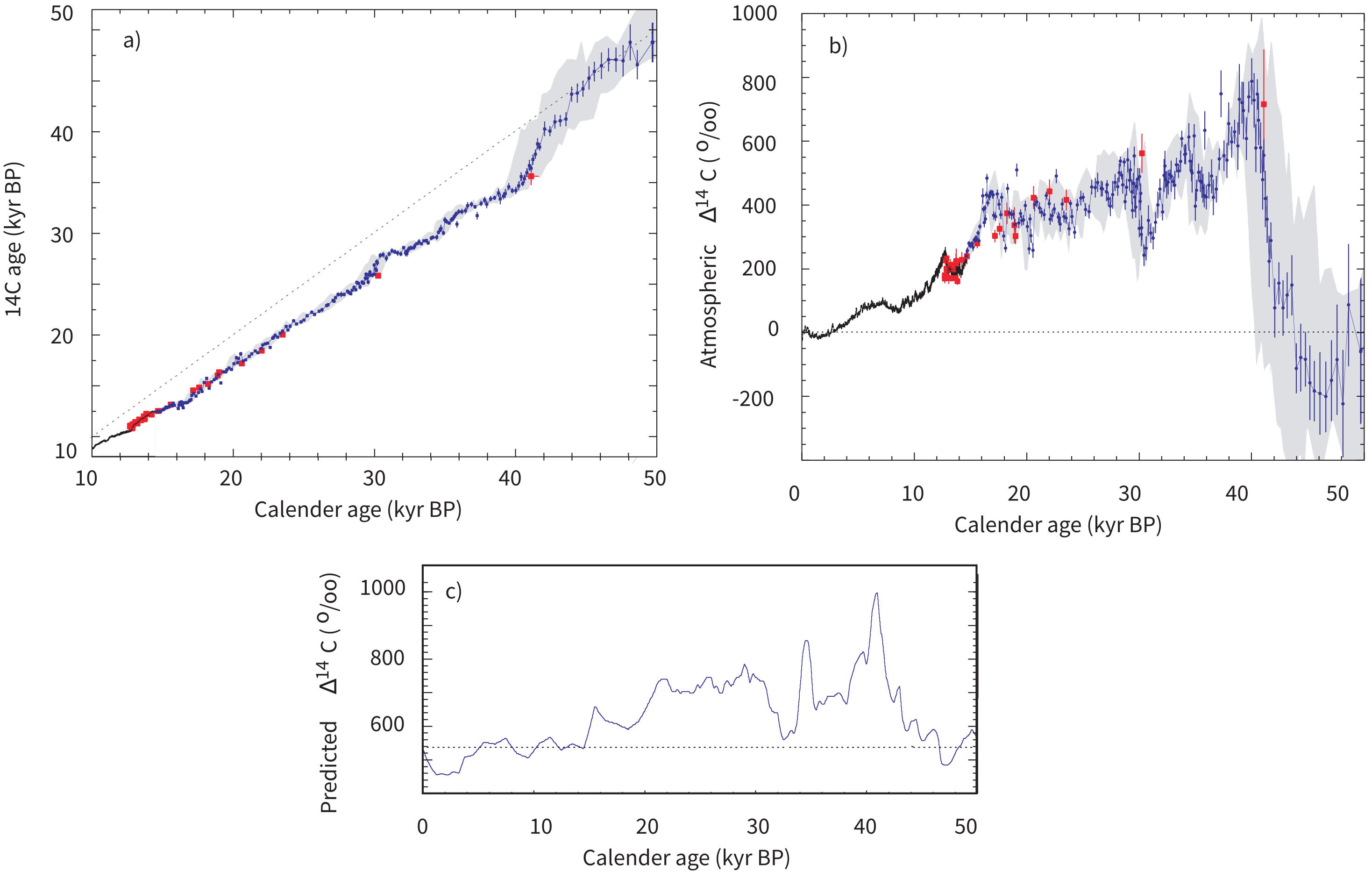
Figure 14.1:a) Radiocarbon calibration data from Cariaco ODP Leg 165, Holes 1002D and 1002E (blue circles), plotted versus calendar age assigned by correlation of detailed paleoclimate records to the Greenland Ice Core GISP2. The thin black line is high-resolution radiocarbon calibration data from tree rings joined at 12 cal. ka B.P. to the varve counting chronology. Red squares are paired C-U/Th dates from corals. Light gray shading represents the uncertainties in the Cariaco calibration. The radiocarbon dates are too young, falling well below the dotted line of 1:1 correlation. b) Compilation of data interpreted as production rate changes in radiocarbon (C) versus calender age. (symbols same as in a). c) Predicted variation of C from the geomagnetic field intensity variations from sediments of the north Atlantic Laj et al., 2002 using the model of Masarik & Beer (1999). [Figure modified from Hughen & others (2004).]
Deep mantle interaction: Studies of seismic waves have demonstrated large variations in seismic velocity near the core mantle boundary. There appears to be an annulus of faster velocities surrounding the Pacific ocean which may reflect the influence of cold subducted slabs. The geomagnetic field is generated by convection in the outer core. This convection could be a strong function of the thermal boundary conditions near the core mantle boundary. Temperature variations in the lowermost mantle therefore could conceivably have an effect on the geomagnetic field (e.g., Glatzmaier et al. (1999)). Is there any evidence for this? Are there any changes in the magnetic field as a function of long term changes in the core mantle boundary?
Inner core interaction: Numerical simulations of the magnetic field predicted that the process of generation of the magnetic field interacted with the inner core in such a way as to make it spin faster than the rest of the Earth Glatzmaier & Roberts, 1996. The effect has been sought in seismic data (e.g., Song & Richards (1996)), although its existence is still a matter of debate.
Tectonic and Geologic applications: Paleomagnetic data often are a critical component of stratigraphic and tectonic investigations because they provide temporal and paleogeographic constraints unavailable by any other method. Therefore, it is useful to know what sorts of data can be expected from records of the geomagnetic field, as oppose to geological modification through initial recording bias, overprinting, or post-formation rotation. It is also useful to know how long one must average the observations to achieve a reasonable estimate of the time averaged field (TAF) and whether or not it can be approximated by a GAD model.
Are we heading toward a reversal?: The Earth’s magnetic field has dropped in intensity since it was first measured. This observation, combined with the fact that the reverse flux patches on the core mantle boundary appear to be growing, lead to speculation that the geomagnetic field might be starting to reverse its polarity (e.g., Hulot et al. (2002)). What is the likelihood that this will happen? What does the field do when it is about to reverse? [Also, what does it do when it is reversing?] What is the average intensity of the field and how frequently does it do what it is doing now without reversing?
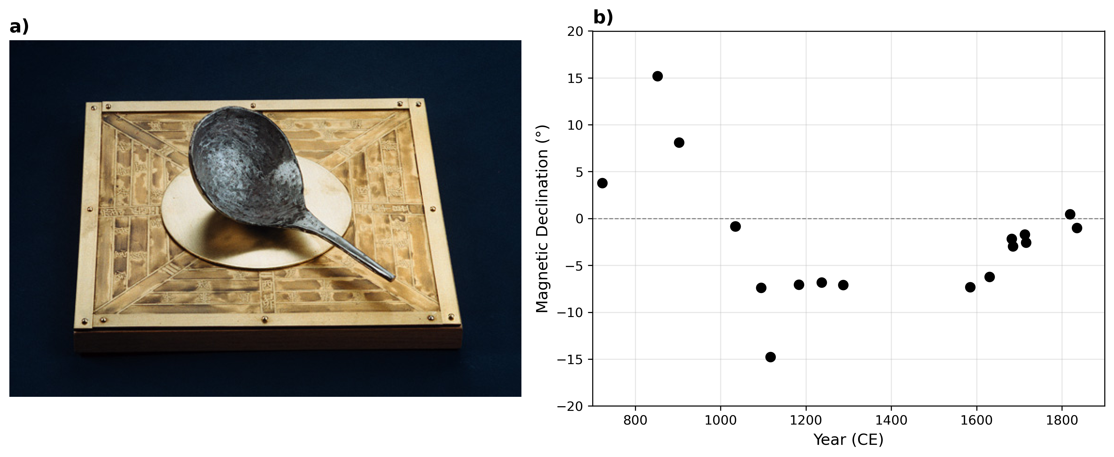
Figure 14.2:a) A reconstruction Wang, 1948 of the south pointing spoon (shao) used by the Chinese in the first century CE. [Photo of Stan Sherer.] b) Measurements of magnetic declination made in China from 720 CE to 1829. [Data quoted in Smith (1967).]
To answer some of the questions just raised, we need measurements of the geomagnetic field. The geomagnetic field changes on frequencies of 10s of microseconds (radio waves) to millions and perhaps billions of years. Direct observations contribute to our knowledge of field behavior for the last few centuries, but on longer times scales we need to use paleomagnetic and archaeomagnetic techniques. We will first review what is known from historical measurements of the geomagnetic field. Then we will turn to what we can glean from accidental records made by archaeological and geological materials.
14.1Historical Measurements
The magnetic properties of lodestone were already well known by the early Greeks. Aristotle (384-332 BCE) wrote of the work of Greek philosopher Thales of Miletos (624-546 BCE) in his book on the soul (De Anima):
Thales, too, to judge from what is recorded about him, seems to have held the soul to be a motive force, since he said that the magnet has a soul in it because it moves the iron.
But the earliest compass appears to date from the first century in China. Lodestone spoons (see Figure 14.2a) were placed on bronze plates, often decorated with images of the Big Dipper and other heavenly images. These “south pointers” were apparently used primarily for prognostication, geomancy and Feng Shui. It was not until sometime in the late 14th Century that compasses were used for sea-going navigation in China.
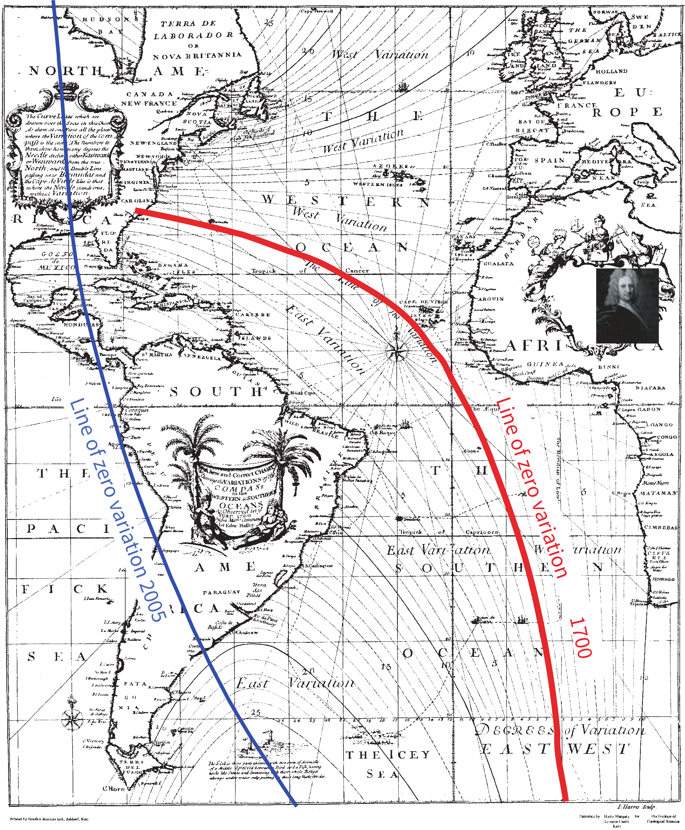
Figure 14.3:Chart of magnetic declination of Halley. Shown in blue is the line of zero variation from the 2005 IGRF. [Figure modified from Cook (2001).]
According to Needham (1962), changes in magnetic declination were discovered in China around 720 CE when the astronomer Yi-Xing measured magnetic declination (see Figure 14.2b). The compass arrived in Europe some time in the 12th century. Magnets and compasses were discussed in a letter (Epistola) by Petrus Peregrinus written in 1269 (finally printed in 1558). Apparently the idea of declination did not accompany the compass. The deviation of magnetic north from true north was not rediscovered by Europeans until the early 1400s. Europeans began to make systematic measurements of declination in the early 1500s. Magnetic inclination was discovered in the mid-1500s in Europe.
Gilbert (1600) noted variations in field strength with latitude based on the sluggishness or rapidity with which a compass settled on the magnetic direction. Magnetic intensity was first measured quantitatively in the late 1700s by French scientist Robert de Paul, although all records were lost in a ship wreck. The expedition sent to search for the lost ship made several measurements, using the period of oscillation of a vertical dip needle with magnetic moment and moment of inertia . These are related to by:
These measurements supported Gilbert’s observation that the intensity of the field increases away from the equator.
The internal origin of the magnetic field was discovered by Gilbert in 1546 who made a systematic study of the magnets and the Earth’s magnetic field, published in 1600. While aware of deviations of magnetic declination from true north, Gilbert thought that the field was unchanging in time. In 1634 Gellibrand compared declination measurements made in London over a period of some 50 years and concluded that the geomagnetic field changes. Thus Europeans discovered secular variation of the magnetic field in 1634, nearly a millenium after the Chinese.
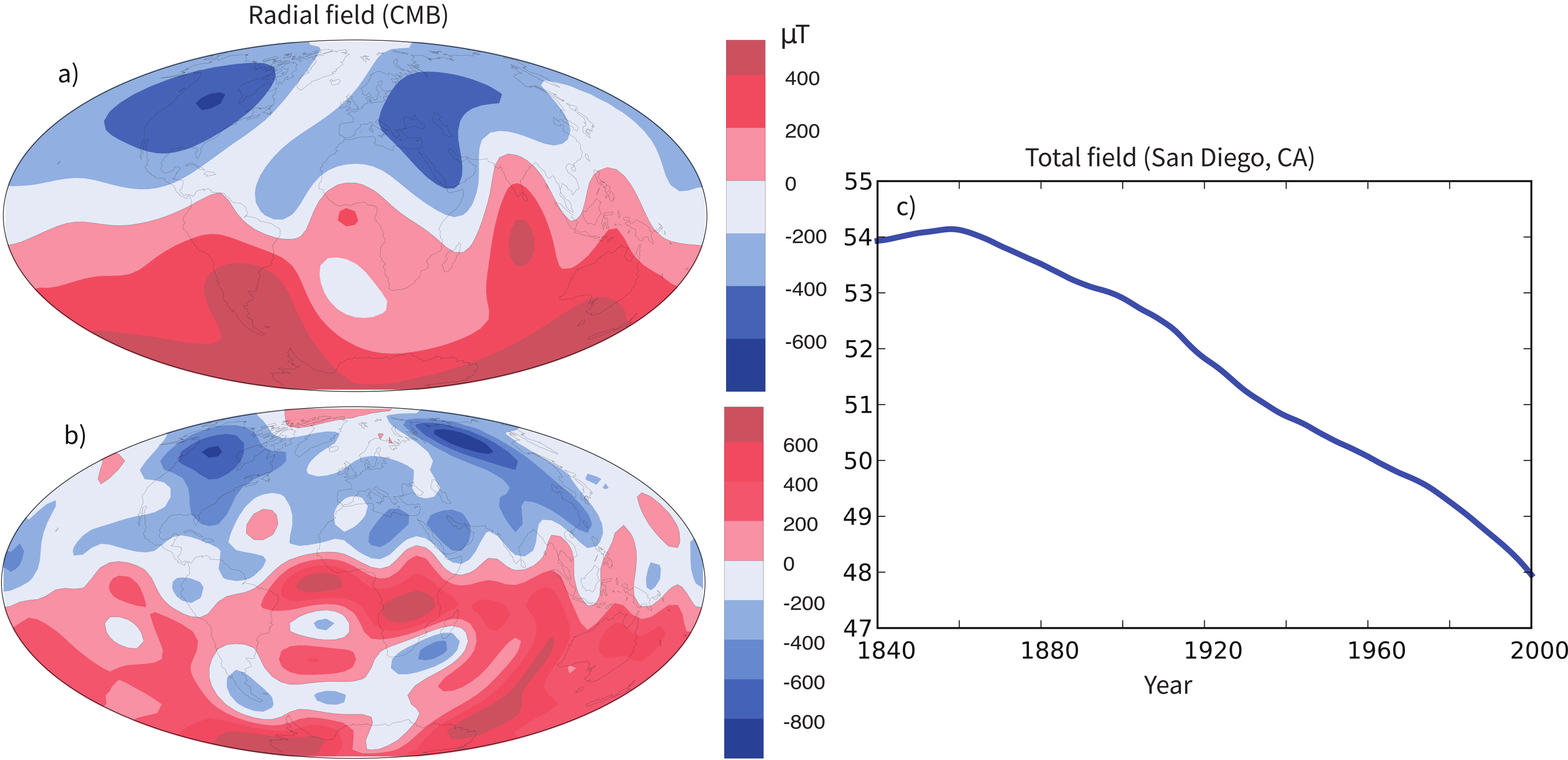
Figure 14.4:Maps of the strength of the radial magnetic field at the core mantle boundary from the GUFM1 secular variation model of Jackson et al. (2000). a) For 1600 CE. b) For 1990. c) Field strength in San Diego, CA evaluated from the GUFM1 model.
Captain Edmond Halley carried out scientific exploration at sea with the expeditions of the Pink Paramore (1698-1701). He produced the first geomagnetic chart (Figure 14.3) sometime between 1700 and 1702 (see Reeves (1918)). Halley noticed that some geomagnetic features appeared to be moving to the west, a phenomenon known as westward drift. Compare for example the “line of no variation” in Figure 14.3 with the line of zero declination from the IGRF of 2005. It has moved significantly to the west in the equatorial and southern Atlantic realms.
Gauss provided the mathematical framework we use today for dealing with geomagnetic data when he derived the spherical harmonic expression for the geomagnetic potential field (see Chapter 2). The first such analysis (done in 1835) was based on 84 data points evaluated on an evenly spaced grid from isomagnetic charts of the magnetic field elements available at the time.
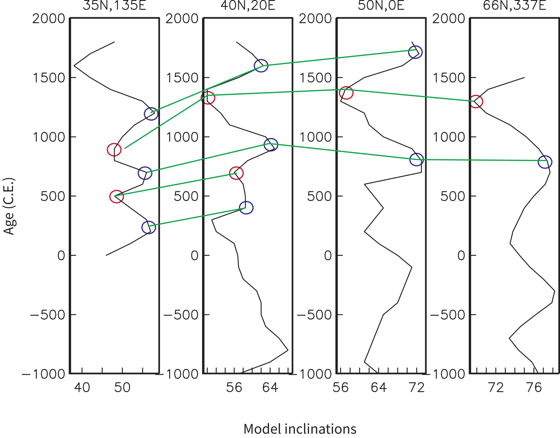
Figure 14.5:Inclinations evaluated at 100 year intervals from the PSVMOD1.0 of Constable et al. (2000) for selected records. These are plotted from East to West. Maxima and minima are noted. Westward drift would imply that these correlated features would “rise” to the right.
Fastforwarding to the current millenium, we find researchers still poring over these centuries old measurements. These ship’s logs contain a huge treasure trove of measurements of declination and sometimes inclination since the 16th century. Such data form the basis for the GUFM1 geomagnetic field model Jackson et al., 2000. The strength of the radial component of the magnetic field inferred for the core mantle boundary at two time intervals in the GUFM1 model is shown in Figure 14.4. Compare Figure 14.4b with Figure 2.4a in Chapter 2 which is the strength of the magnetic field observed at the surface. There are more so-called flux patches (the spots of higher intensity) in Figure 14.4b because the field was evaluated closer to the source (the core), but the general pattern is similar. The field for 1600, however, was somewhat different. The number and positions of the flux patches has changed substantially since then. Some flux patches, in particular the prominent patch that is now over Africa, have moved from the Indian ocean, a phenomenon largely responsible for westward drift.
As already mentioned, observatory measurements of the intensity of the magnetic field are only available since the mid-19th century. These show that the large changes in declination and inclination were also accompanied by even more dramatic changes in field strength. We plot the intensity of the field evaluated from the GUFM1 model for San Diego, CA, in Figure 14.4c. If the field continues on its recent trajectory, it will reach zero by the year 2500.
14.2Archaeo- and Paleomagnetic Records
Historical observations quickly run out as we go back in time. Prior to 720 CE there are no surviving human measurements. Yet the average field based on the historical measurements (e.g., Jackson et al. (2000)) is clearly not GAD. To see how observations of the magnetic field such as westward drift, quasi-stationary flux lobes and the degree of “GADness” change through time, we must turn to rock and archaeological materials to give us a picture of the ancient geomagnetic field.
14.2.1Pioneers in Paleomagnetism
Strongly magnetized rocks (as opposed to the mineral lodestone) had been noticed during the 1700s because of their effect on compass needles, but the fact that certain rocks were magnetized in the direction of the Earth’s field was discovered by Delesse in 1849 and Melloni in 1853. Folgheraiter (1899) extended the study of fossil magnetizations to the magnetic properties of baked archaeological materials in 1899. Naturally baked material (heated by lava flows) was studied by David (1904) and Brunhes (1906). In the course of their investigations, they discovered materials adjacent to normally magnetized rock that were magnetized in a direction opposite to the Earth’s field. This first application of the baked contact test led to speculation that the Earth’s field had reversed its polarity in the past. Mercanton (1926) argued that the field had reversed polarity because reversely magnetized rocks were found all over the world. Matuyama (1929) further supported the argument by demonstrating that all the reversely magnetized rocks in Japan were older than the overlying normally magnetized rocks. It was not until the combined use of paleomagnetism and K-Ar dating allowed researchers in the U.S. and Australia (e.g., Cox et al. (1963); McDougall & Tarling (1963)) to demonstrate the global synchrony of polarity intervals that the scientific community embraced the notion of polarity reversals.
Sedimentary materials were first used for the investigation of secular variation by Johnson et al. (1948) who measured samples from varved lakes in New England. Mackereth developed a pneumatic coring device for use in lakes in 1958, opening the way for studies of the detailed time variations of the magnetic field.
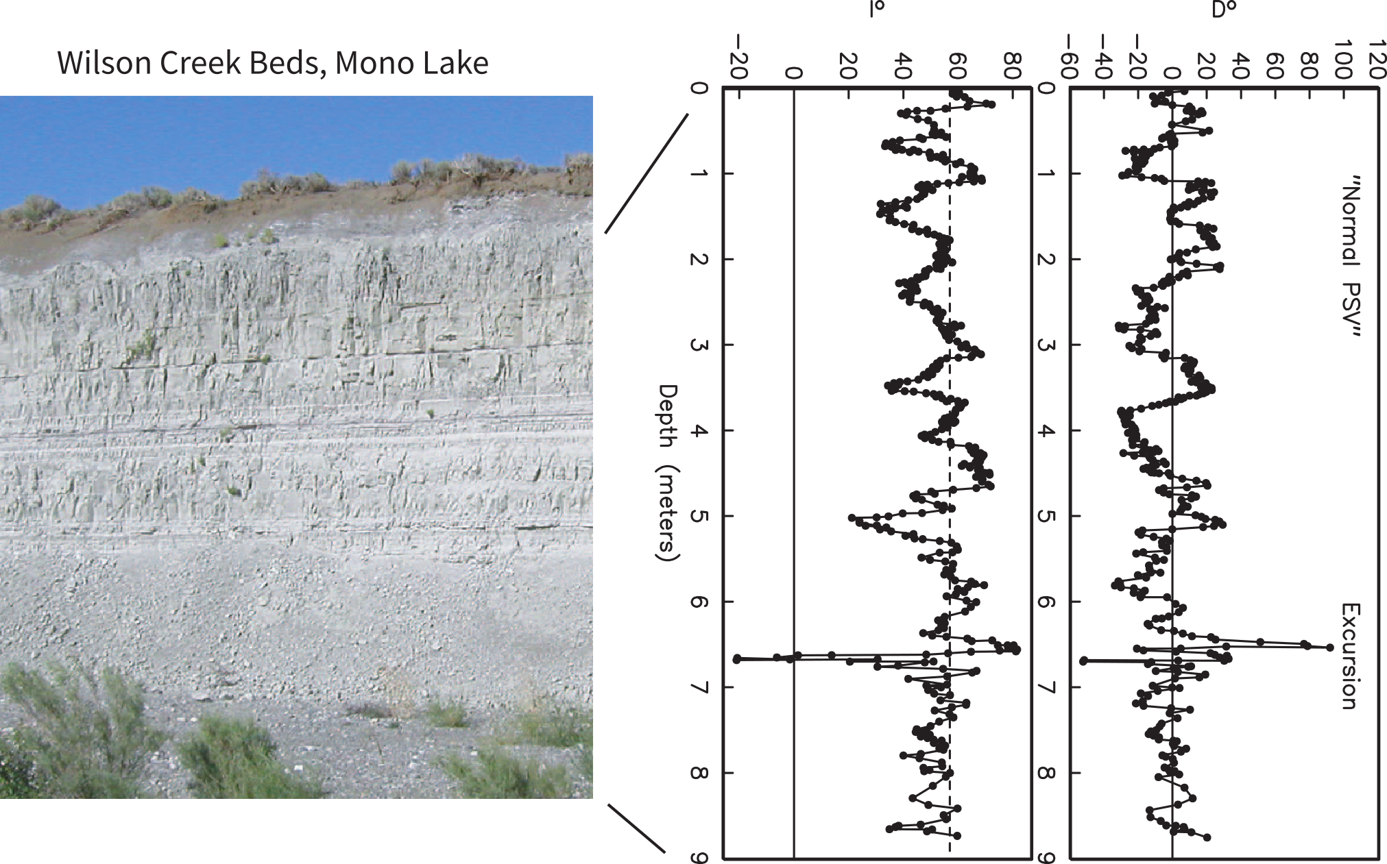
Figure 14.6:Paleosecular variation of the magnetic field ( and ) observed in the Wilson Creek section north of Mono Lake. The inclination expected from a geocentric axial dipole is shown as a dashed line. The declination is expected to be zero. The so-called “Mono Lake” excursion is marked. The data are from Lund et al. (1988) and represent some 23 kyr of time.
14.2.2The Last Seven Millenia
Spherical harmonic models that push back our understanding of geomagnetic field behavior to times without deliberate, systematic human measurements rely on compilations of archaeomagnetic and paleomagnetic data. Constable et al. (2000) assembled a data set of 24 time series of directional data from archaeomagnetic and lake sediment sources evaluated at 100 year intervals (PSVMOD1.0). We plot examples of several of the inclination records from East to West in Figure 14.5.
These efforts were significantly advanced by the inclusion of archaeological and volcanic data sets which resulted in a series of models of the form CALSxK.n (e.g., Korte & Constable (2003); Korte & Constable (2005)). The name stands for “Continuous models of Archaeomagnetic and Lake Sediment data for the past x thousand years, version n.” The first model of this series, CALS3K.1 Korte & Constable, 2003 included no intensity information, while a more recent version, CALS7k.2, relies on the data compilation of Korte et al. (2005) including directional and intensity data from archaeological, sedimentary and volcanic sources spanning the last seven millennia.
The CALS7K.2 model can be used for a wide range of studies (see Korte & Constable (2008)). For example, we can begin to answer questions such as the control of the geomagnetic field on production of cosmogenic nuclides, or millennial scale variability in the geomagnetic dipole. Geomagnetic field vectors can be predicted for a given place at a given time. Predictions from paleosecular variation “master curves” are frequently used to provide constraints for archaeomagnetic dating (see, e.g., Lanos et al. (2005)) and more accurate field models of the CALSxK style will improve such constraints considerably.
New data compilations are being published every year (e.g., the Geomagia50 database of Korhonen et al. (2008) and ArchaeoInt database of Genevey et al. (2008)). With these new comprehensive data collections, improved models will be constructed for longer time series. This is a fast moving field, so stay tuned.
14.2.3Westward Drift
We mentioned that early workers measuring the secular variation of declination noticed that certain features appeared to move west with time. A careful look at the data shows that this tendency is a subtle, probably only locally observed effect. Yukutake (1967) collected together the data available at the time and marked the occurrences of maxima and minima in both declination and inclination. Some of these are marked on Figure 14.5 as examples. Yukutake then plotted these maxima and minima as a function of age and longitude of the observation site. The data appeared to suggest that the features moved westward at a rate of about a half a degree per year. This would mean that the maxima and minima on Figure 14.5 would rise to the right as they sort of do, but the data are rather unconvincing.
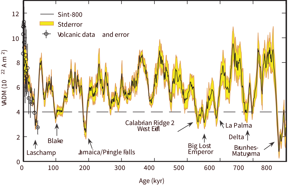
Figure 14.7:Stack of relative paleointensity records from deep sea sediments. [Figure modified from Guyodo & Valet (1999).]
14.2.4The More Distant Past
For more distant times in the past, accurate chronological constraints become difficult and direct comparison of geomagnetic features globally becomes more difficult. Field models of the GUFM and CALSxK type which predict geomagnetic field vectors for any place at any time become increasingly more difficult to constrain. Nonetheless, there are important questions that can be addressed.
For example:
Secular variation over the last few millennia has involved factor of two changes in geomagnetic field strength and directional variability of tens of degrees. How does the geomagnetic field behave over longer time intervals? How strong can the field get? How fast can it change?
The geomagnetic field is clearly not entirely dipolar, yet much of paleomagnetic research relies on the assumption that on average the geomagnetic field is that of a geocentric axial dipole. How much time must be averaged for this to be a good approximation?
There are two approaches to studying the geomagnetic field in ancient times: examination of time series from data for which chronological ordering is known and estimating statistical properties of the paleomagnetic field. In the following sections we will consider first what we have learned from the time series approach and then we will turn to statistical models.
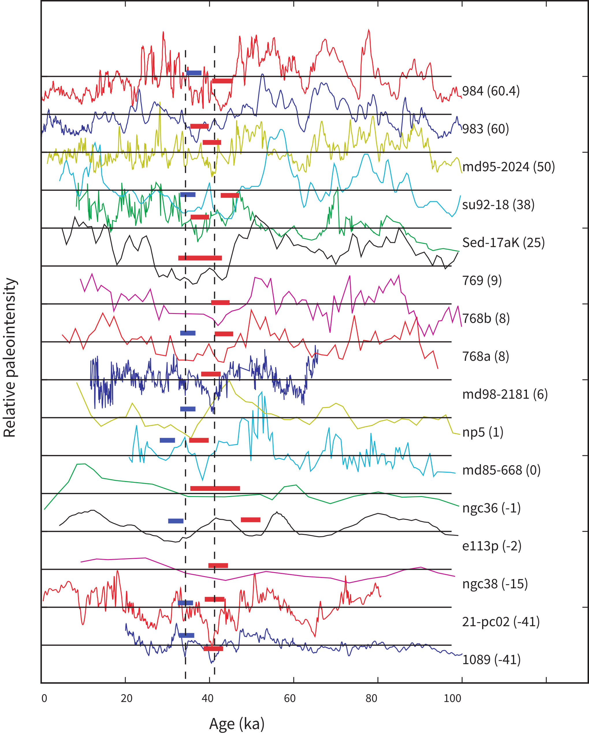
Figure 14.8:Relative paleointensity records spanning the last 100 kyr with independent age control based on O. The solid red bars indicate intensity lows that are possibly related to the “Laschamp excursion” and the blue bars are a later paleointensity low, referred to as the “Mono Lake excursion”. [Figure from Tauxe & Yamazaki (2007).]
14.3Time Series of Paleomagnetic Data
14.3.1Excursions
In Figure 14.6, we see an example of a detailed record of the geomagnetic field, obtained from dry lake sediments exposed along the shores of Mono Lake in California. The geomagnetic field oscillated around the direction expected from a GAD field over an interval of some 9 meters. The amplitude of directional variability is generally contained within about 30° of the GAD direction. At about 6.75 m, however, the field direction departed drastically from that, achieving a nearly antipodal direction. This type of behavior is known as a geomagnetic excursion.
The definition of a geomagnetic excursion is problematic. The traditional definition identifies magnetic records in which the VGPs are more than 45° away from the average pole for that time and place as excursional. As we shall see in Section 14.7, the scatter in VGPs may depend on latitude with higher scatter at higher latitudes. Basing the identification of an excursion on a given VGP cut-off angle then means that more excursions will be identified at higher latitudes.
In a recent review of the phenomenon on excursions, Laj & Channell (2007) advocated that the term be used for features that represent departures from “normal” secular variation, for which a full polarity reversal has not been established. This usage is quite vague, relying on an undefined concept of what is “normal”. They introduced the term microchron for brief polarity intervals. These would exhibit fully reversed directions and would presumably be globally observed. Other definitions of the term “excursion” have been used implicitly. For example, excursions are thought to be accompanied by a decreases in paleointensity (DIPs) (a paleointensity low). For this reason, some studies (e.g., Guyodo & Valet (1999)) have identified “excursions” based on the occurrence of paleointensity lows (see Figure 14.7). The rationale for this lies in the fact that most “deviant” directions that have paleointensity data associated with them, have “low” values (see Section 14.3.2).
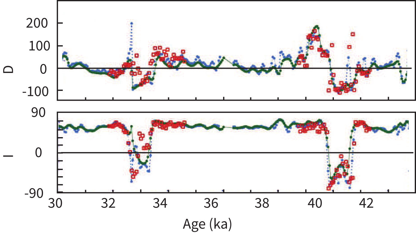
Figure 14.9:Directional data from ODP Site 919. Declination () and inclination () data from continuous core (“u-channel”) measurements (dark/green closed symbols connected by line), deconvolved u-channel data (closed gray/blue symbols connected by dashed line) and data from 1cc discrete samples (open/red squares without connecting line). [Figure redrawn from Channell (2006).]
We name excursions after the place where it was first observed, so the one documented in Figure 14.6 is known as the Mono Lake excursion. This presupposes that the Mono Lake excursion is unique from other excursions requiring a global assessment of excursions and their ages. The age of the Mono Lake record has been hotly contested. Kent et al. (2002) argue that it is approximately 38-41 ka, which is quite similar to the age of another famous excursion, the Laschamp excursion, discovered in volcanics near Laschamp, France (see Bonhommet & Zähringer (1969) and references therein; see also Plenier et al. (2007) for recent review of the Laschamp data).
Dating sedimentary sequences like the Mono Lake is difficult, but so is dating very young lava flows like the Laschamp volcanics because of the low abundance of radioactive potassium. Zimmerman et al. (2006) weighed in on the issue using relative paleointensity data from the Wilson Creek section (shown in Figure 14.6) and concluded that the data agree best with relative paleointensity data unequivocally associated with the Laschamp excursion. Cassata et al. (2008) report new Ar/Ar ages ranging from 31.6±1.8 ka to 39.1±4.1 ka for a set of volcanic rocks in New Zealand from which “excursional” directions and low paleointensities had been obtained (e.g., Shibuya et al. (1992); Cassidy (2006); Mochizuki et al. (2006)). Cassata et al. (2008) claim that there are two excursions represented in these lavas and tie them to the Mono Lake and Laschamp excursions, although there is no volcanic stratigraphy to provide independent proof. The question as to whether there are in fact two independent excursions is unresolved by these data.
Resolution of the Mono Lake-Laschamp mystery therefore lies in records with stratigraphic age control. One such record is the paleointensity proxy record of Cl and Be data in Greenland ice cores (GRIP and GISP cores). The advantage of ice cores is that not only is the relative chronology straight-forward, layer counting in the ice gives ages that are accurate to within 60 years. The isotopes Cl and Be are produced in the atmosphere by cosmic ray bombardment which is modulated by the geomagnetic field strength and the strength of the solar wind. Therefore changes in production rate of these isotopes reflects to a large extent reflect changes in intensity of the field. The isotopic data from the Greenland Summit cores were summarized by Muscheler et al. (2005). The Be flux data do not show two peaks, but a single peak centered at approximately 39 ka. The Cl data, however are less straight-forward. The data differ in two papers published in the same year on the same core by the same group Wagner et al., 2000Wagner et al., 2000. One of these has two peaks, centered on ~31 and ~39 ka respectively, while the other has but a single peak at ~39 ka.
Another way of addressing the Mono Lake-Laschamp dilemma would be to look at the sedimentary relative paleointensity database. Tauxe & Yamazaki (2007) compiled nearly all of the published relative paleointensity records. Data with independent O age control spanning the last 100 kyrs are shown in Figure 14.8. DIPs at around ~40 and ~30 ka are marked with red and blue bars. These have been interpreted as representing the “Mono Lake” and “Laschamp” excursional paleointensity lows. While a few records appear to have both, the evidence is not overwhelming for two globally recorded features.
Finally, we have the directional records from sedimentary sequences long enough to record both excursions. Channell (2006) published a detailed record with adequate independent age constraints from oxygen isotopes spanning the 30 to 42 kyr interval of interest (see Figure 14.9). There are two distinct excursional intervals in this record, one at ~33 ka and the other at ~40 ka. This core comes from quite close to another core, SU92-18, whose relative paleointensity is shown in Figure 14.8 and is one of the cores with two distinct paleointensity lows.
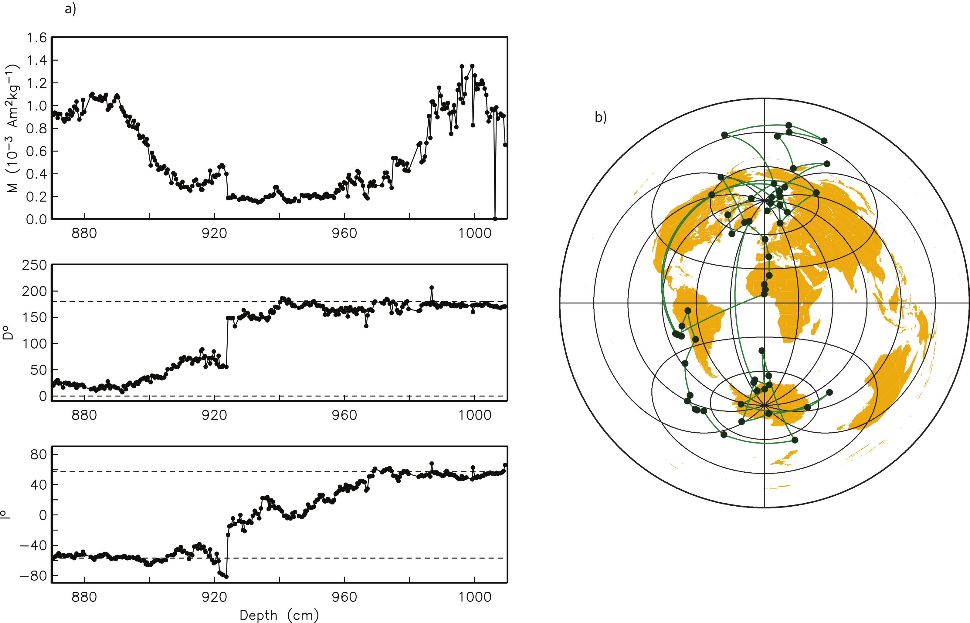
Figure 14.10:a) The lower Jaramillo geomagnetic polarity reversal as recorded in deep sea sediments from core RC14-14. Inclinations and declinations expected from a normal and reverse GAD field are shown as dashed lines. [Data from Clement & Kent (1984).] b) Record of polarity transition recorded at Steens Mountain. [Data from Camps et al. (1999).]
The conclusion from all these different perspectives is that while there may be two excursions at about ~30 and ~40 ka respectively, it is still not clear whether these are global features and which of these the sediments at Mono Lake itself actually recorded. The conservative interpretation would be that there is a globally observed feature with nearly fully reversed directions and low paleointensity values at about ~39 ± 2 ka observed in France, California and New Zealand. Associated low paleomagnetic intensity values at about this time are also observed at in the Greenland ice cores (by Be proxy) and many deep sea sediment cores (Figure 14.8). This feature should properly be called the “Laschamp” and if we adopt the terminology of Laj & Channell (2007), it would be classified as a microchron. It is also clear from the recent literature, that there is no consensus as to what the term “excursion” means. Laj and Channell (2007) reserve the term for what are essentially local phenomena that do not reach fully antipodal directions. By this measure, the feature occasionally observed at about ~30 ka would be an excursion. Because this was first well documented as being a directional feature distinct from the Lashamp in the Irminger Basin Channell, 2006, perhaps it should be named the Irminger Basin excursion.
We have examined in detail only a few of the many directional and intensity aberrations that have been called “excursions” over the years. Each has its own history and many may turn out to be as interesting and difficult to pin down as the Mono Lake-Laschamp feature(s).
14.3.2Reversals
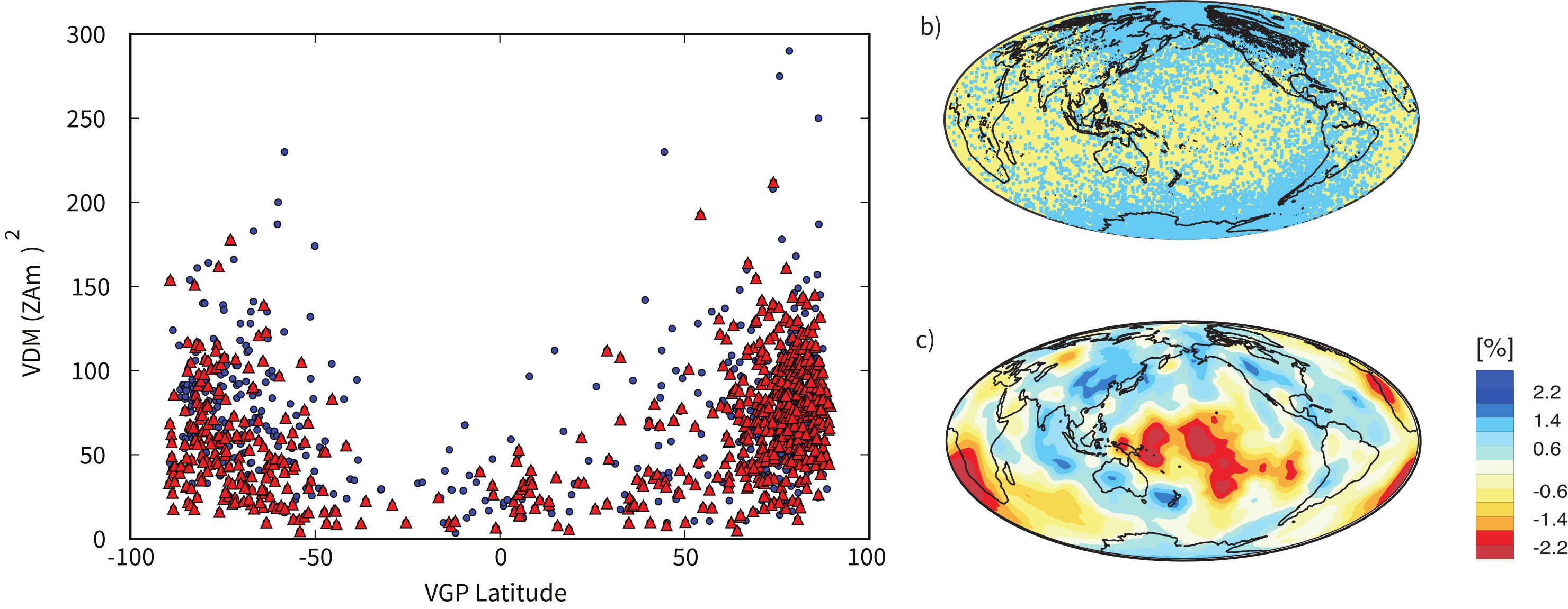
Figure 14.11:a) VDM versus VGP latitude from data in the PINT06 database compiled by Tauxe & Yamazaki (2007). The red triangles are from double heating experiments with pTRM checks (see Chapter 10). b) Plot of transitional VGPs (blue dots) from the TRANS data base McElhinny & Lock, 1996. No selection criteria were applied. c) Shear wave velocity SB448 model of Masters et al. (2000) evaluated at 2770 km (core mantle boundary region). There is a fast (cold) ring around the Pacific, presumably from the influence of subducted slabs.
When viewed over sufficient time, the geomagnetic field reverses its polarity, by which we mean that the sign of the axial dipole term () changes. An example of a paleomagnetic record of a polarity reversal is shown in Figure 14.10a Clement & Kent, 1984. The intensity of the magnetic field appears to drop to approximately 10% of its average value and the directions migrate from one pole to the other over a period of several thousand years. When the polarity is the same as the present polarity it is said to be normal. When it is in the opposite state, it is said to be reverse. The duration of the reversal process also appears to be a function of latitude Clement, 2004.
The details of what happens during a polarity reversal are still rather unclear because they occur so quickly, geologically speaking. Some high resolution sedimentary records are like that shown in Figure 14.10 whereby there is an orderly progression from one polarity to the other. However, a polarity transition captured by rapidly erupted lava flows records a more complex picture (see Figure 14.10b). There are a few conclusions we can draw however: 1) they occur quickly and 2) they are always associated with low geomagnetic intensities (see Figure 14.11a).
A more controversial observation about directions in extrema was first pointed out by Clement (1991); when mapped to VGP positions, they plot in preferred longitudinal swaths (see Figure 14.11b). These swaths are seen in many data sets, but can be made to disappear when certain criteria are applied (e.g., Prévot & Camps (1993)). The intriguing thing about the swaths is that they appear to coincide with the shear velocity anomalies in the lowermost mantle suggesting some control of the temperature structure near the core mantle boundary on structure of the paleomagnetic field (see Figure 14.11c). Whether or not the swaths exist has been debated ever since they were first observed.
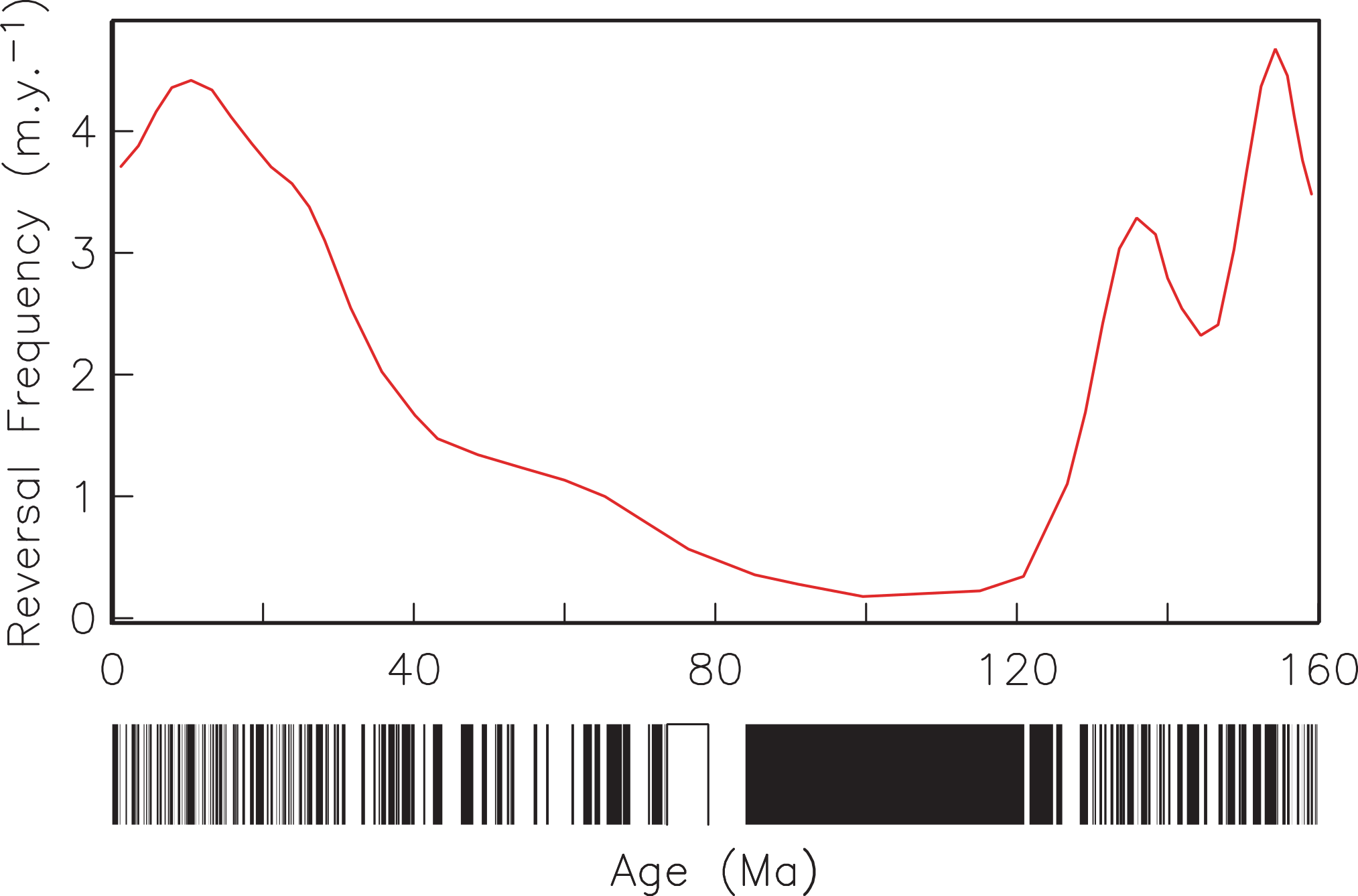
Figure 14.12:Barcode: The Geomagnetic Polarity Time Scale (GPTS) for the last 160 Ma Berggren et al., 1995Gradstein et al., 1995. Line traces the reversal frequency (number of reversals in a four million year interval) estimated by Constable (2003).
On average, the field spends about half its time in each polarity state, and only a tiny fraction (1-2%) of the time in an intermediate state. Rocks of both polarities have been documented from early in the Earth’s history (at least since the late Archean, see Strik et al. (2003)), although the frequency of reversal has changed considerably through time (see Opdyke & Channell (1996) and Merrill et al. (1996)).
14.4Geomagnetic Polarity Time Scale -- A First Look
A list of dates of past geomagnetic polarity reversals is known as a geomagnetic polarity time scale (GPTS). How the time scale is calibrated is discussed in the next chapter. For now we will just take it as a given. In Figure 14.12 we show the polarity history from the marine magnetic anomaly template. The details of the history of reversals for times older than the oldest sea floor magnetic anomaly record (about 160 Ma) are sketchy, but will eventually be documented using sedimentary records of the magnetic field (see e.g., Kent & Olsen (1999)).
Examination of the reversal history shown in Figure 14.12 suggests that reversals occur at apparently random intervals without a predictable pattern. Furthermore, the frequency of reversals appears to change (see for example, Constable (2003)). Above the polarity history in Figure 14.12, we plot the reversal frequency estimated by Constable (2003). The reversal frequency is relatively high in the interval 124-150 Ma, but appears to drop gradually to zero at the beginning of the so-called Cretaceous Normal Superchron (CNS), a period of some 38 Myr in which no (or very few) reversals occurred. Since the end of the CNS at about 83 Ma, the frequency of reversals has increased to the present average rate of about four per million years.
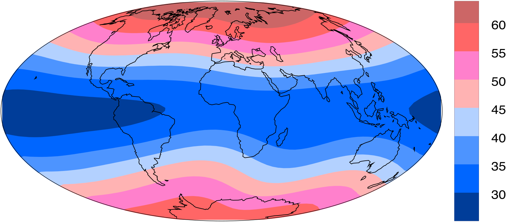
Figure 14.13:Time averaged intensity of the geomagnetic field. [Model of Hatakeyama & Kono (2002).]
14.5The Time Averaged Field
In Sections Section 14.1 and Section 14.2 we reviewed several field models that were time series of full scale spherical harmonic models. Beyond a certain age limit, however, there simply are not enough data with sufficient age control and spatial density to constrain a spherical harmonic model. The approach for longer time scales has been to look at the average magnetic field or the statistical characterization of paleosecular variation data. We consider here the time averaged field.
The last five million years has been a focus for time average field models because the effects of plate motion are small and there are hundreds of studies to draw from. Data from lava flows from all over the world have been compiled into various databases and analyzed from a variety of view points. It was recently realized that the data had been compiled using less than optimum criteria and that many more data of higher overall quality may be required for a robust TAF model to be produced. Data from the new TAF project are only just becoming available (e.g., Johnson et al. (2008)). In the mean time, we show a plot of the TAF model of Hatakeyama & Kono (2002) in Figure 14.13. Although the field is not perfectly GAD, the flux patches seen in the historical field are nearly erased.
One of the primary assumptions in many paleomagnetic studies is that the magnetic field, when averaged over sufficient time, averages to that of a GAD field. This means that if VGPs are averaged from units spanning enough time to average out secular variation, the mean pole is coincident with the spin axis. Such a pole is called a paleomagnetic pole. As continents move, they carry with them rock units that retain a record of the spin axis in the continental reference frame, so these poles tend to form swaths called apparent polar wander paths or APWPs. We will learn more about APWPs in Chapter 16. It is worth mentioning here that it is not very well known exactly how much time is required to average out secular variation; the consensus is that it is more than 400 years but less than 5 million. Most text books claim that 10--10 years is sufficient. The minimum number of sampling sites required for a “good” average is also poorly constrained. Conventional wisdom suggests at least ten, while Tauxe et al. (2003) suggest that approximately 100 sites are required to fully sample secular variation.
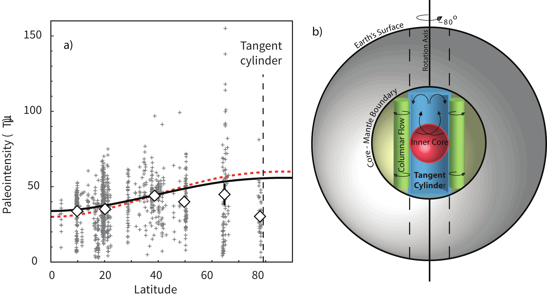
Figure 14.14:a) Paleointensity versus latitude of the Pint06 database (grey crosses) (see Tauxe & Yamazaki (2007)) and paleointensity estimates from Lawrence et al. (2009) for data with ages less than 5 Ma, 15 T, and 2. Mean paleointensity results (diamonds) are calculated for 15° latitude bins and errors are shown as 2. The black line is the longitudinal-averaged intensity for today’s field. The vertical dashed line is the surface expression of the edge of the tangent cylinder. Southern hemisphere data have been flipped to the Northern hemisphere. The black line represents the mean intensity for today’s field as defined by the 2005 IGRF model coefficients, while the red dashed line represents the intensity associated with a geocentric axial dipole with a dipole term of 30 T. b) Illustration of outer core flow regimes. The tangent cylinder is denoted by the blue cylinder tangential to the red sphere (inner core). [Figures redrawn from Lawrence et al. (2009).]
Another aspect of secular variation and the time averaged field is the variation and average strength of the field. Tauxe & Yamazaki (2007) updated the PINT03 database of Perrin & Schnepp (2004) to include all published paleointensity data through 2006. We show site-averaged paleointensity estimates (grey crosses) derived from the updated paleointensity database in Figure 14.14a. We also include the new data from Antarctica of Lawrence et al. (2009). The only filter for selecting PINT06 data was that the number of samples had to be at least two and the standard deviation of the site mean intensity had to be less than or equal to 15%. Southern hemisphere data are combined with the Northern hemisphere to decrease latitudinal gaps. To reduce the effects of regional variations, the site-level estimates are averaged in 15° latitude bins (diamonds) with 95% confidence levels calculated using a bootstrap.
One puzzling feature of Figure 14.14a is the absence of an increasing trend in the intensity data with latitude. An axial dipole field would have polar intensities twice those expected at the equator, and although for the present field non-axial dipole contributions reduce this gain somewhat (as shown by the solid black line), all conventional wisdom suggests that we would expect the average field strength to increase (double) with latitude. Also shown in Figure 14.14a (dashed red line) is field expected from a geocentric dipole with the strength 80 ZAm. Neither of these two curves describe the trend in the available data, which if anything suggest weakening of the field above 65°.
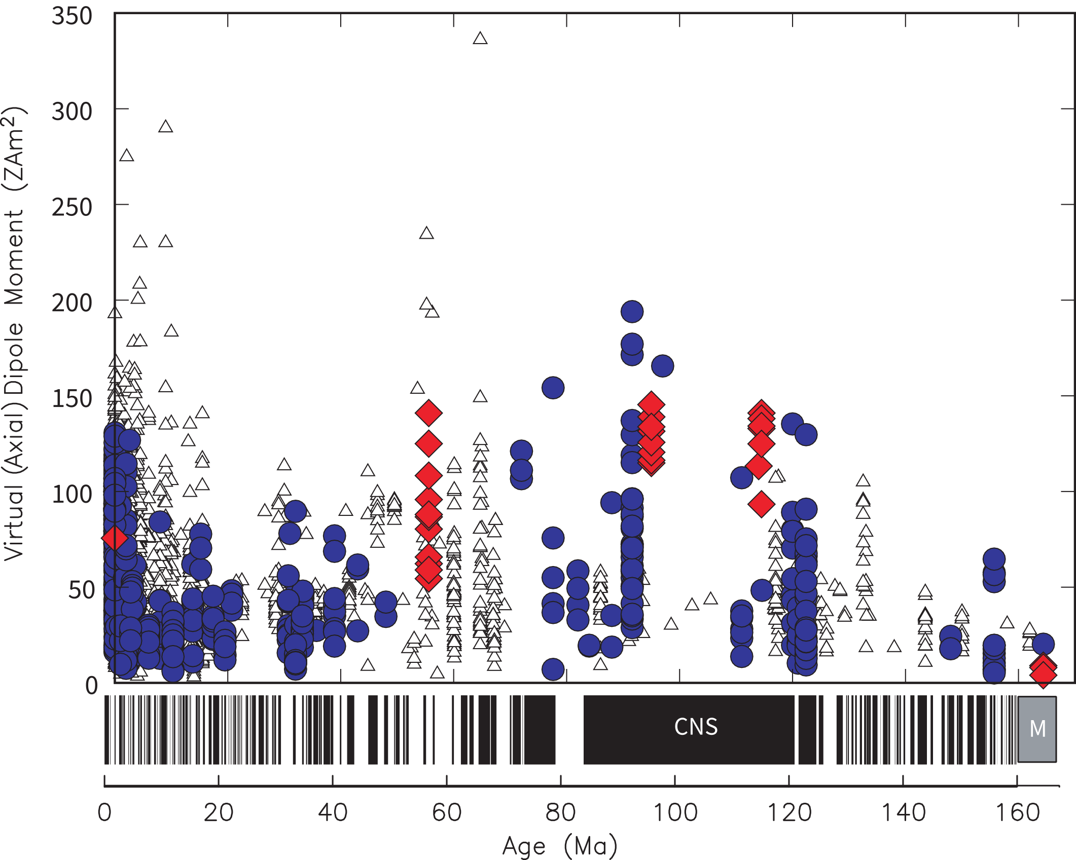
Figure 14.15:Summary of data in the PINT06 compilation of Tauxe & Yamazaki (2007) meeting minimum acceptance criteria for last 200 Ma. Blue dots are submarine basaltic glass data. Red diamonds are single crystal results. Triangles are all other data meeting the same consistency criteria ( 5% of mean or 5T). At the bottom is the Geomagnetic Polarity Time Scale showing the Cretaceous Normal Superchron (CNS) and the M-sequence of magnetic anomalies. [Figure from Tauxe & Yamazaki (2007).]
The apparent trend in intensity might arise from inadequate temporal and geographic sampling of the geomagnetic field Lawrence et al., 2009. Or, it is possible that the influence of the inner core manifests itself in lower average field strengths at and above the cylinder tangent to it (the tangent cylinder). The geodynamo results from a complex combination of physical processes in the fluid outer core (see, e.g., Merrill et al. (1996)). The influence of the Coriolis force, combined with the presence of the inner core results in a separation of the flow regimes into two distinct regions bounded by a cylinder tangent to the inner core, parallel to the spin axis. (e.g, Aurnou et al. (2003); see Figure 14.14b). The spin of the Earth tends to generate columnar convection in the region outside the tangent cylinder, while inside, the convection tends to be more 3-dimensional Busse, 1983. It is possible that the flow regime inside the tangent cylinder results in a depressed field strength observed at high latitude.
14.6Long Term Changes in Paleointensity
We plot a compilation of paleointensity data since the Jurassic in Figure 14.15, from Tauxe & Yamazaki (2007). Early compilations suggested that much of the Mesozoic had a rather low field intensity (the Mesozoic dipole low of Prévot et al. (1990)) with an apparent average intensity of about 25% of the present field which is ~80 ZAm. The more recent compilation of high quality paleointensity data by Tauxe & Yamazaki (2007) shows that the Cenozoic also had a moderate field, suggesting that the Mesozoic “dipole low” is probably a common state of the geomagnetic field, with anomalously high values occurring in the latter part of the Cretaceous and early Cenozoic and during the last few thousand years.
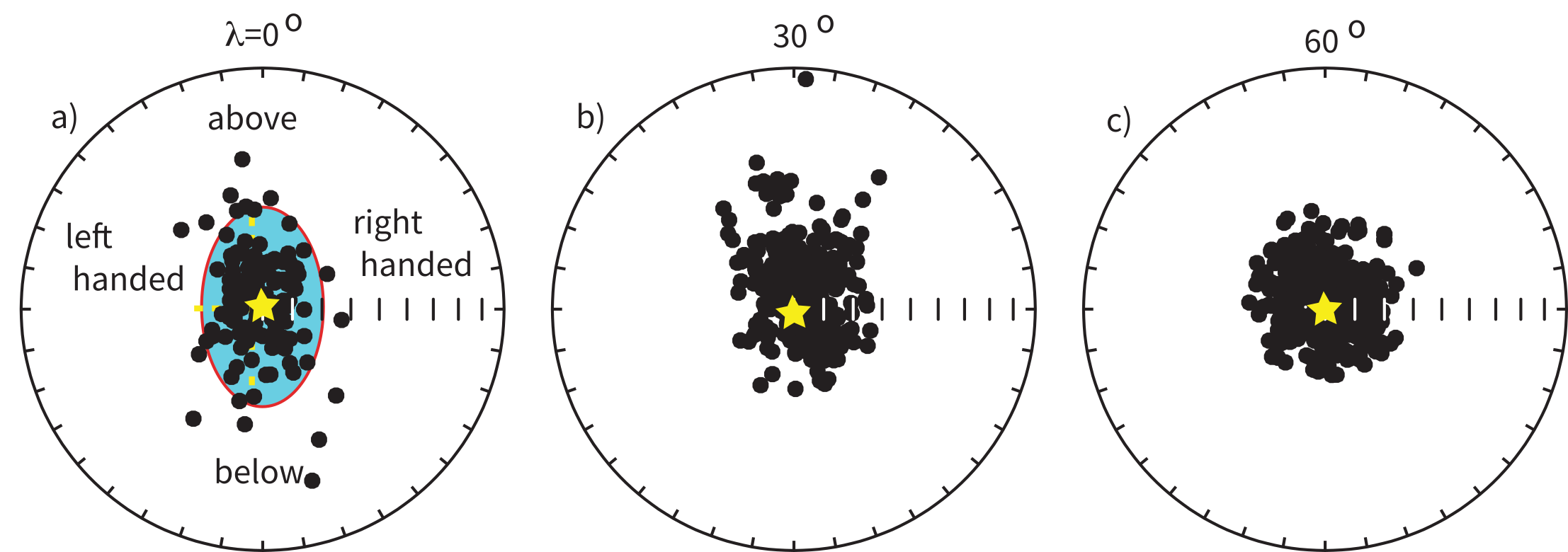
Figure 14.16:a) Paleomagnetic directions from the PSVRL database (see McElhinny & McFadden (1997)) compiled for latitude band 0-5° (N&S). Antipodes of reverse directions are used. The expected direction is at the star at the center of the equal area projection. Directions in the upper (lower) half are above (below) those expected and those to the right (left) are right-handed (left-handed). The red ellipse illustrates the elongation of the directional data where is the ratio of the eigenvalues along the maximum and minimum axes (here vertical and E-W respectively). b) Same as a) but for 25-35° (N&S) latitude band. c) Same as a) but for 55-65° (N&S) latitude band. [Figures redrawn from Tauxe & Kent (2004).]
14.7Statistical Models of Paleosecular Variation
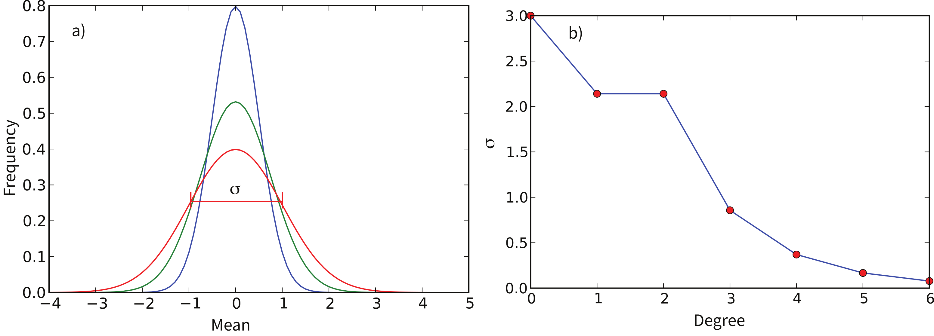
Figure 14.17:a) Illustration of a normal distribution with varying standard deviations. b) Variation of standard deviation as a function of spherical harmonic degree in the CP88 model.
From studies of the time averaged field it seems that, at least for the last five million years, the field has been dominantly that of a geocentric axial dipole (GAD). At any particular instant in time, however, there will be significant deviations owing to the non-axial dipole contributions. This, combined with distortions in the recording process (some of which were discussed in Chapter 5) and decreasing preservation of rocks with increasing age makes evaluating the GAD hypothesis increasingly difficult as we go back in time.
There has been considerable effort in collecting the data relevant to describing the statistical character of the geomagnetic field over time. Selected results from one such collection (that of McElhinny & McFadden (1997); MM97) are shown in Figure 14.16. Directions from lava flows less than five million years old from particular latitudinal bands are plotted with respect to the expected GAD direction at that particular latitude ( from Chapter 2).
Several things are worth mentioning about the data in Figure 14.16. First, it appears that the equatorial data are more elongate than those from higher latitudes (something we mentioned in Chapter 12). The elongation parameter can be used to quantify this and is the ratio where are the eigenvalues of the orientation matrix (see Section A.3.5.4). Secondly, the scatter in the directional data seems to go down with increasing latitude. Thirdly, when the directions are converted to VGPs, the dispersion in VGPs tends to increase with latitude.
Before we begin a quick tour of PSV models, we must introduce the concept of VGP scatter and briefly explain how it has been calculated. VGP scatter is quantified by the parameter (e.g., Cox (1969)), defined as:
where is the number of observations and is the angle between the VGP and the spin axis.
Ideally, one would use all the paleomagnetic data available, but we encounter two problems with this approach. First, some directions are better determined while others have significant within site scatter resulting from sampling or experimental errors (or lightning strikes!). Secondly, the interest of the paleomagnetic community in unusual field states (reversals and excursions) has resulted in their over-representation in the published literature.
To address the issue of within site scatter, some studies use a cutoff for or for inclusion in the calculation, while others adjust the value of to account for the within site scatter . McElhinny & McFadden (1997) defined a parameter :
where is the average number of samples per site.
To address the over-representation of unusual field states in the data base, some data compilations have used a fixed cutoff for VGP latitude. For example, the MM97 database culled data with VGP latitudes at 45° away from the poles. The latitudinal dependence of means that a fixed cutoff biases against the more scattered data collected at higher latitude. This bias results in a rather peculiar distribution of directions for the high latitude sites (Figure 14.16c). In an attempt to compensate for this problem, Vandamme (1994) proposed a variable VGP cutoff. The Vandamme cutoff () is found using a recursive method such that , where is the value of for the trimmed data set.
Most early modeling efforts by the paleomagnetic community focussed on explaining the variable scatter in directions and VGPs with latitude (see review by Tauxe & Kodama (2009)). The first model of secular variation of the Earth’s magnetic field is the dipole wobble model of Creer et al. (1959). This has become known as Model B Irving & Ward, 1963. Dipole wobble (simulated by random variations in the three dipole terms of the spherical harmonic expansion of the geomagnetic field) produces Fisher distributed sets of virtual geomagnetic poles (VGPs). These are centered around the spin axis. Because of the non-linear transformation from VGPs to directions (see Chapter 2 and Chapter 12), the directions associated with a circularly symmetric set of VGPs are not generally circular.
A different PSV model, Model A of Irving & Ward (1963), starts from Fisher distributed directional data modeled by adding directional perturbations drawn from a uniform distribution to the expected dipole direction. The VGP distribution resulting from such a process would be oval at the equator and become more circular toward the poles.
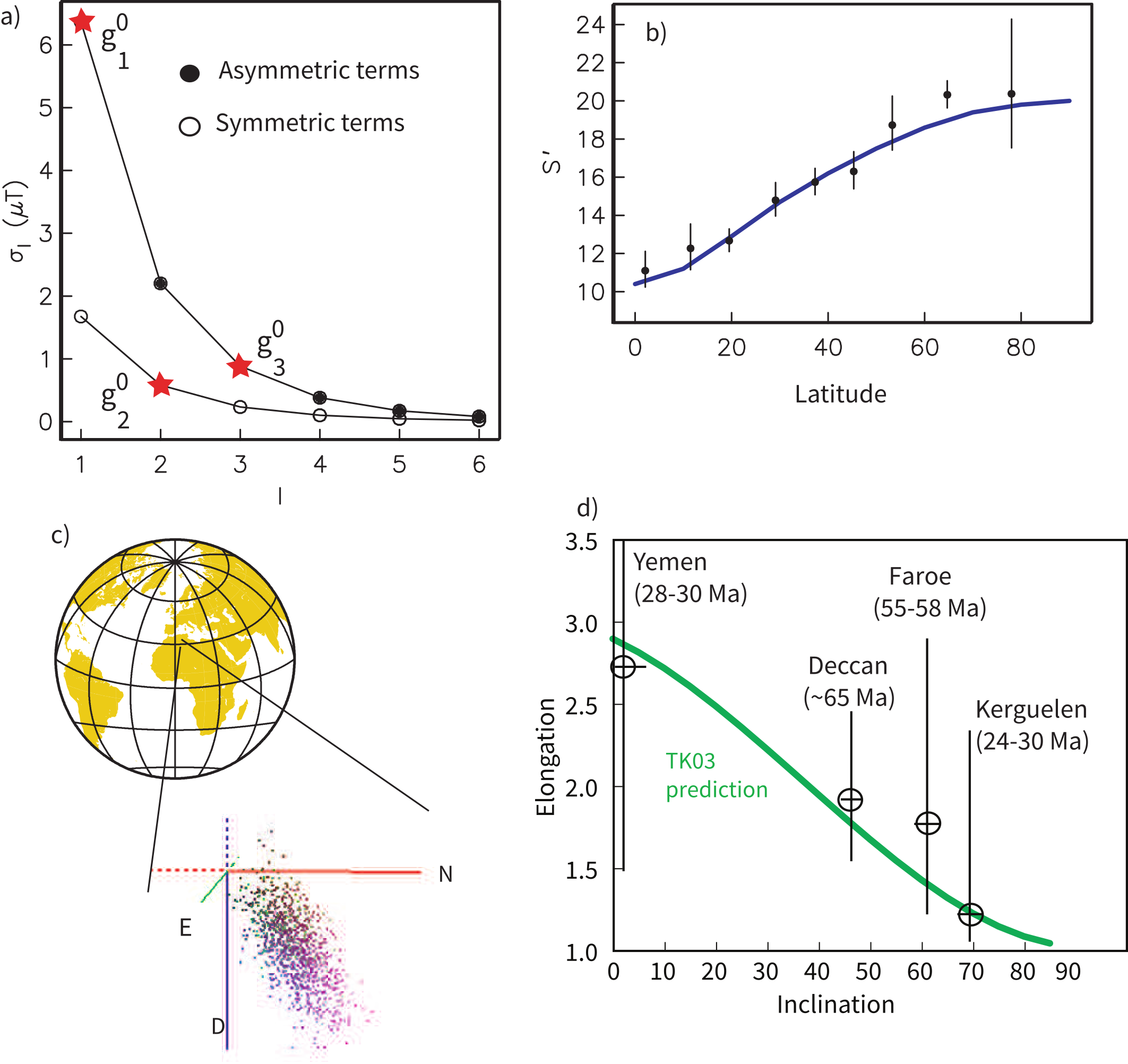
Figure 14.18:a) Variation of the standard deviation as a function of harmonic degree for asymmetric and symmetric terms for the statistical field model TK03.GAD. All terms have zero mean except the axial dipole term. b) Estimated behavior of from the data compilation of McElhinny & McFadden (1997) (circles). Blue line is the predicted variation of from the TK03.GAD model of Tauxe & Kent (2004). c) 1000 vector endpoints from realizations of model TK03.GAD at 30°N. d) Elongation versus inclination predicted from the TK03.GAD model. Compilation of data from LIPs of Tauxe & Kodama (2009). Crossed open circles are data from large igneous provinces back through time. Yemeni traps: Riisager et al. (2005). Deccan traps: Vandamme et al. (1991); Vandamme & Courtillot (1992). Faroe Island basalts: Riisager et al. (2003). Kerguelen: Plenier et al. (2002). [Figures from Tauxe & Kent (2004); Tauxe (2005); Tauxe & Kodama (2009).]
Model G of McFadden & McElhinny (1988) modeled the increasing VGP scatter with latitude by separating the geomagnetic field into the “dipole” and “quadrupole” families described by Roberts & Stix (1972). In the dipole family, the Gauss coefficients () produce fields that are antisymmetric about the equator (those with odd) while in the quadrupole family, the Gauss coefficients produce fields that are symmetric about the equator (those with even). The antisymmetric terms contribute more strongly to scatter in VGPs with latitude than the symmetric terms. Model G thus has the form:
where and are the antisymmetric and symmetric family coefficients, respectively and is latitude. McElhinny & McFadden (1997) found that values of and provided a good fit to their “better quality” dual polarity data set representing the last five million years.
Paleosecular variation models of the form of Equation 14.4 predict average VGP scatter as a function of latitude. This is but one of the many interesting and useful observations about the statistical behavior of the magnetic field and it would be wonderful if we had a way of predicting for a given latitude the full vector distributions expected from the geomagnetic field. To find a “full service” statistical paleosecular variation model, we begin with the work of Constable & Parker (1988) (hereafter CP88). The CP88 statistical paleosecular variation model assumes that the time varying geomagnetic field acts as a “Giant Gaussian Process” (GGP) whereby the gauss coefficients (see Chapter 2) (except for the axial dipolar term, and in some models also the axial quadrupole term ) have zero mean. The standard deviations (see Figure 14.17a) are a function of degree and a fitted parameter (as in Figure 14.17b), and, for , follow the formula:
where is the ratio of the core radius to that of Earth (0.547). Many data sets show a persistent offset in equatorial inclinations at least in reverse polarity data sets, consistent with a small non-zero mean axial quadrupolar term (). We are ignoring this effect here because it is in all studies a small term.
In the GAD version of CP88 in which , once the average dipole moment , its standard deviation and are fixed, realizations of field models can be created by drawing the gauss coefficients from their respective gaussian distributions. Geomagnetic vectors can then be calculated for any given location using the usual transformation from the geomagnetic potential equation to geomagnetic elements (see Chapter 2).
The principal drawback of the CP88 model is that it fails to fit the observed scatter in the paleomagnetic data with latitude. Most of the subsequent variations on this theme attempted to address the VGP scatter problem by introducing more fitted parameters, losing the elegant simplicity of the CP88 model.
The most recent model of the statistical paleosecular variation genre is the TK03.GAD model of Tauxe & Kent (2004); see also Tauxe & Kodama (2009). Like CP88.GAD, TK03.GAD has only three parameters: (set to fit a recent estimate for the long term average intensity of the axial dipole as in Figure 14.15), as defined in CP88, but fit to the more recent compilation of directional data of McElhinny & McFadden (1997) and a new paramter which is the ratio of the asymmetric ( odd) to the symmetric ( even) gauss coefficients for a given . We show the variation in with degree for the two families (asymmetric and symmetric) in Figure 14.18a. The term allows a much improved fit to the paleomagnetic observations (see Figure 14.18b) while the model retains the simplicity of the CP88 model. Please note that a new generation of models is on the way that will incorporate the vast amount of new data being generated (for a preview of things to come, see Johnson et al. (2008)).
In Figure 14.18c we show the vector end points calculated from 1000 realizations of the model at 30°N. The distribution of these vectors predicts what would be observed at that latitude if we had a large number of observations of the geomagnetic field or its paleomagnetic proxies.
Models like TK03 can predict the distribution of geomagnetic field vectors at any location. These, then, can be compared with the observed paleomagnetic data in order to assess whether the data are consistent with the field model. The TK03 model was designed to predict values for in agreement with those observed in the PSVRL database (see Figure 14.18b), but there are other attributes of the field that can be predicted as well. For example, while inclination can be calculated from the simple dipole formula (see Chapter 2) for any latitude, the elongation of the directions (e.g., Figure 14.16a) requires a statistical field model. In fact, because elongation goes down with increasing latitude, while inclination goes up, there is a unique elongation/inclination pair that is consistent with a given statistical field model. The elongation/inclination trend calculated from the TK03.GAD model is shown in Figure 14.18d.
Data from the last five million years fit the model predictions as it was designed to do, but the model can be tested through time by calculating the elongation/inclination pair for data sets of any age. The requirements are that the data are referenced to paleo-horizontal, that the directions represent the ancient geomagnetic field (they are not biased by overprinting, inclination error, etc.), and that there be a sufficient number to represent the statistical variability of the ancient geomagnetic field. There are not many data sets that satisfy these requirements. Tauxe & Kodama (2009) compiled data sets from ancient large igneous provinces that did: the Deccan Traps in India Vandamme et al., 1991Vandamme & Courtillot, 1992, the Faroe Island basalts Riisager et al., 2003, and Kerguelen Plenier et al., 2002. The elongation/inclination pairs from these data sets are plotted on Figure 14.18d for comparison with the model predictions. It appears that the TK03.GAD model can be used as a guide to the geomagnetic field behavior for at least the Tertiary.
SUPPLEMENTAL READINGS: Tauxe & Kodama (2009); Johnson et al. (2008).
14.8Problems
Problem 1
You learned how to use the function ipmag.igrf in the problems for Chapter 2. The program uses the official DGRF and IGRF field models since 1945. A special feature of the program, however, is the use of the GUFM1 coefficients of Jackson et al. (2000) for dates between 1600 and 1945. Note that while ipmag.igrf only calculates a single date at a time we can easily set up a list with results for a time series.
a) Calculate the variation in inclination of the geomagnetic field in Sicily (latitude of 38°, longitude of 14°E) between 1600 and 1900 (at 10 year intervals) and make plots of the field elements using the matplotlib plotting utility. Use the most recent data model available.
b) The GUFM1 coefficients were estimated using deliberate, human observations. An independent data set is that from lava flows and archaeological artifacts. These can be searched using the GEOMAGIA web set at http://
c) Find the Rolph et al. (1987) paper in the geomagia data set as an example. and read the paper. Are the data reliable? Make an equal area plot of the directions in the geomagia download file. Do they look ok?
Problem 2
Paleointensity data have been assembled into databases for quite some time. A recent version of the compilation is from this website: http://
a) Find all the VDM/VADM estimates for the last 10 Myr. Select the data that were done with a Thellier double heating type experiment, with pTRM checks (T+) and those that were done with the Shaw method (S). Plot the VDM/VADMs from both sets versus age. Are there any differences?
b) Now find all the T+ data that have polarity information for the last 10 Myr. Separate the data into N, R, and T groups. Plot these versus age (with different symbols). Are there any differences?
Problem 3
The dependence of scatter in directions and VGPs on latitude is well known.
a) Go to the MagIC database website and download the data for one high latitude data set (Lawrence et al. (2009)): Lawrence et al. (2009)
Create a Project Directory and put the file in it. Unpack it with ipmag.download_magic.
b) Read in the site mean data from the sites.txt file into a Pandas DataFrame, knowing that the files are always tab delimited and have a header in the second line (header=1 to Pandas). Look at the directions in equal area projection using the ipmag.plot_net and ipmag.plot_di functions from within your Jupyter notebook. Be sure to get rid of all the blank directional data (MagIC headers of dir_dec, dir_inc with the Pandas function dropna.
Plot the VGPs with ipmag.plot_vgp. To do that, you will need to have Basemap installed. Follow the instructions in the help message to make a simple map. As this is a dual polarity data set, first make an nested [lon,lat] array and use pmag.flip to separate it into normal and verse antipodes. Be sure to drop all the records with no VGP data in them (using Pandas dropna function) first.
c) Write a program that will calculate the VGP scatter statistic from VGPs. What is of the entire data set? [Use the antipodes of the reverse data.]
d) Now modify your program to calculate as a function of latitude cutoff, i.e., make an option to exclude VGP latitudes with latitudes more than a specified amount away from the spin axis. What is the “best” latitude cut-off?
e) A file called hawaii.txt is stored in the Chapter_14/Problem_3 directory. This is a compilation of all the data from Hawaii used in a recent analysis of the time averaged field project by Cromwell et al. (2018). Repeat problems 2b-d on the Hawaiian data set. Is there a latitude dependence of ?
f) Compare these values of to those predicted by Model G.
Problem 4
a) Use the program ipmag.tk03 to generate a nested list of 100 vectors for a latitude of 20° (the approximate latitude of Hawaii). Plot them using the functions ipmag.plot_net, ipmag.plot_di. Hint, it would be easiest to turn the output of ipmag.tk03 into an array and take the transpose. Then the first element is an array of declinations and the second is the inclinations.
b) Find the present IGRF and GAD directions at 20° and -156° using the functions ipmag.igrf and pmag.pinc. Rotate the directions in hawaii.tk03 to the expected GAD direction using the function pmag.dodirot_V. Hint: try the nice NumPy function column_stack to put your directions into the right format. Plot these rotated directions using the ipmag functions. Now rotate the directions extracted from hawaii.txt in Problem 2e plot them in equal area projection. How do the directions predicted by the PSV field model compare with the data set from Hawaii?
c) Use the function pmag.doprinc to calculate the eigenparameters of the orientation matrix of the Hawaiian directions (see Chapter 9 and Section A.3.5.4). What is wrong with either the GAD model or the data set?
- Kono, M. (Ed.). (2007). Treatise on Geophysics, Volume 5: Geomagnetism. Elsevier.
- Merrill, R. T., McElhinny, M. W., & McFadden, P. L. (1996). The Magnetic Field of the Earth: Paleomagnetism, the Core, and the Deep Mantle. Academic Press.
- Laj, C., Kissel, C., Mazaud, A., Channell, J. E. T., & Beer, J. (2002). North Atlantic paleointensity stack since 75 ka (NAPIS-75) and the duration of the Laschamp event. Philosophical Transactions of the Royal Society of London A, 358, 1009–1025. 10.1098/rsta.2000.0571
- Masarik, J., & Beer, J. (1999). Simulation of particle fluxes and cosmogenic nuclide production in the Earth’s atmosphere. Journal of Geophysical Research: Atmospheres, 104(D10), 12099–12111. 10.1029/1998JD200091
- Hughen, K. A., & others. (2004). Marine04 marine radiocarbon age calibration, 0-26 cal kyr BP. Radiocarbon, 46(3), 1059–1086. 10.1017/S0033822200033002
- Glatzmaier, G. A., Coe, R. S., Hongre, L., & Roberts, P. H. (1999). The role of the Earth’s mantle in controlling the frequency of geomagnetic reversals. Nature, 401, 885–890. 10.1038/44776
- Glatzmaier, G. A., & Roberts, P. H. (1996). Rotation and magnetism of Earth’s inner core. Science, 274(5294), 1887–1891. 10.1126/science.274.5294.1887
- Song, X., & Richards, P. G. (1996). Seismological evidence for differential rotation of the Earth’s inner core. Nature, 382, 221–224. 10.1038/382221a0
- Hulot, G., Eymin, C., Langlais, B., Mandea, M., & Olsen, N. (2002). Small-scale structure of the geodynamo inferred from Oersted and Magsat satellite data. Nature, 416, 620–623. 10.1038/416620a
- Wang, C. T. (1948). Discovery and application of magnetic phenomena in China. 1. The lodestone spoon of the Han. Chinese Journal of Archaeology, 3, 119.
- Smith, P. J. (1967). The intensity of the ancient geomagnetic field: a review and analysis. Geophysical Journal of the Royal Astronomical Society, 12(4), 321–362. 10.1111/j.1365-246X.1967.tb03146.x
- Cook, A. (2001). Edmond Halley and the magnetic field of the Earth. Notes and Records of the Royal Society of London, 55(3), 473–490. 10.1098/rsnr.2001.0159
- Needham, J. (1962). Science and Civilisation in China, Volume 4: Physics and Physical Technology, Part 1: Physics. Cambridge University Press.
- Jackson, A., Jonkers, A. R. T., & Walker, M. R. (2000). Four centuries of geomagnetic secular variation from historical records. Philosophical Transactions of the Royal Society of London A, 358(1768), 957–990. 10.1098/rsta.2000.0569
- Reeves, E. A. (1918). Edmond Halley’s chart of magnetic variation. The Geographical Journal, 51(4), 237–241. 10.2307/1780108