In Chapter 4, we discussed the energies that control the state of magnetization within ferromagnetic particles. Particles will tend to find a configuration of internal magnetization directions that minimizes the energies (although meta-stable states with local energy minima or LEMs are a possibility). The longevity of a particular magnetization state has to do with the depth of the energy well that the magnetization is in and the energy available for hopping over barriers.
The ease with which particles can be coerced into changing their magnetizations in response to external fields can tell us much about the overall stability of the particles and perhaps also something about their ability to carry a magnetic remanence over the long haul. The concepts of long-term stability, incorporated into the concept of relaxation time, and the response of the magnetic particles to external magnetic fields are therefore linked through the anisotropy energy constant (see Chapter 4) which dictates the magnetic response of particles to changes in the external field. This chapter will focus on the response of magnetic particles to changing external magnetic fields.
5.1The “flipping” field
Magnetic remanence is the magnetization in the absence of an external magnetic field. If we imagine a particle with a single “easy” axis — a so-called “uniaxial” particle with magnetic anisotropy constant , the magnetic energy density (energy per unit volume) of a particle whose magnetic moment makes an angle to the easy axis direction (Figure 5.1a) can be expressed as:
As the moment swings around with angle to the easy axis, the anisotropy energy density will change as plotted in Figure 5.1b. The energy minima are when is aligned parallel to the easy axis (an axis means either direction along the axis, so either 0° or 180°). In the absence of a magnetic field, the moment will lie along one of these two directions. In reality, thermal energy will perturb this direction somewhat, depending on the balance of anisotropy to thermal energy, but for the present discussion, we are assuming that thermal energy can be neglected.
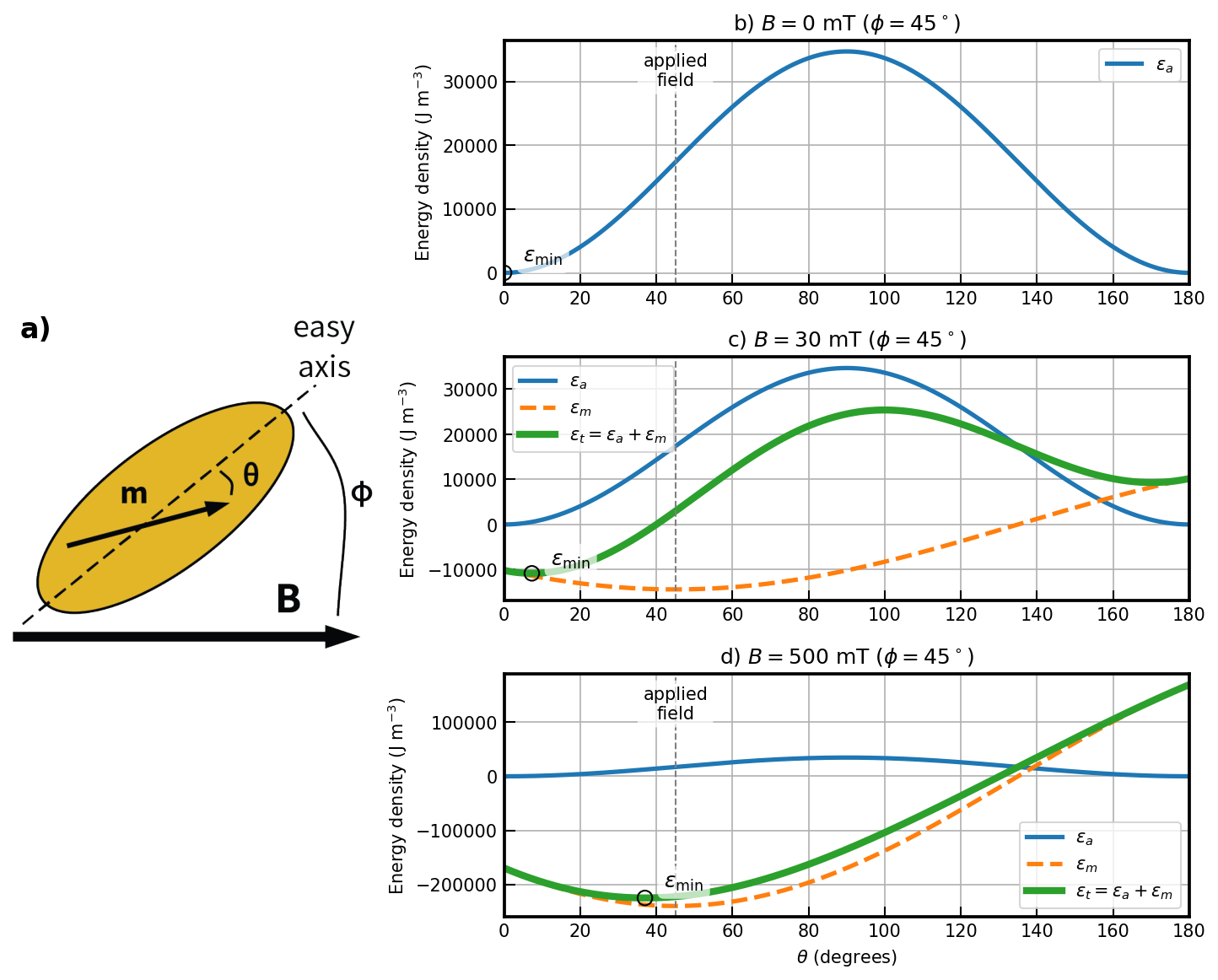
Figure 5.1:a) Sketch of a prolate spheroid magnetic particle (magnetite, elongation q = 2) with easy axis along the long dimension. In response to a magnetic field , applied at an angle to the easy axis, the particle moment rotates, making an angle with the easy axis. b) Variation of the anisotropy energy density () as a function of . The energy is minimized along the easy axis () and the highest perpindicular to that axis. c) Applying a field of B = 30 mT at a as shown in (a) leads to interaction energy density () as shown by the orange dashed line. The anisotropy energy density () is the same as in (b) with the total energy density being the two added together (). The effect is for the grain magnetization to be slightly pulled away from the easy axis as indicated by the position of the energy minimum (). d) Applying a larger field of 500 mT, results in domiance of the interaction energy density that pulls the energy minimum () much closer to the applied field direction.
When an external field is applied at an angle to the easy axis (and an angle with the magnetic moment; see Figure 5.1a), the magnetostatic interaction energy density () is given by the dot product of the magnetization and the applied field (Equation 4.2 in Chapter 4):
The two energy densities ( and ) are shown as the thin solid and dashed lines in Figure 5.1c for an applied field of 30 mT aligned with an angle of 45° to the easy axis. There is a competition between the anisotropy energy (tending to keep the magnetization parallel to the easy axis) and the interaction energy (tending to line the magnetization up with the external magnetic field). Assuming that the magnetization is at saturation, we get the total energy density of the particle to be:
The total energy density is shown as the heavy solid line in Figure 5.1c,d.
The magnetic moment of a uniaxial single domain grain will find the angle that is associated with the minimum total energy density (; see Figure 5.1). For low external fields, will be closer to the easy axis (e.g., 30 mT in Figure 5.1c) and for higher external fields will be closer to the applied field direction ((e.g., 500 mT in Figure 5.1d)).
When a magnetic field that is large enough to overcome the anisotropy energy is applied in a direction opposite to the magnetization vector, the moment will jump over the energy barrier and stay in the opposite direction when the field is switched off. The field necessary to accomplish this feat is called the flipping field () (also sometimes the “switching field”). [Note the change to the use of for internal fields where cannot be considered zero.] We introduced this parameter in Chapter 4 (see Equation 4.14) as the microscopic coercivity. Stoner & Wohlfarth (1948) showed that the flipping field can be found from the condition that and = 0. We will call this the “flipping condition”. The necessary equations can be found by differentiating Equation 5.3:
and again
Solving these two equations for and substituting for , we get after some trigonometric trickery:
where . In this equation, is the angle between the applied field and the easy axis direction opposite to .
The interactive visualization below demonstrates the flipping field for a prolate spheroid magnetite particle (aspect ratio ). The magnetization starts aligned with the easy axis opposite to the applied field. You can use the slider to gradually increase the applied field and observe how the energy landscape evolves. The magnetization stays in a local energy minimum until the magnetization flips to align with the applied field in the global energy minimum. This flip happens the energy barrier goes away, which corresponds to when the second derivative of the total energy curve goes to zero.
Now we can derive the so-called “microscopic coercivity” () introduced in Section 4.1.6 in Chapter 4. Microscopic coercivity is the maximum flipping field for a particle. When magnetic anisotropy of a particle is dominated by uniaxial anisotropy constant and is zero (antiparallel to the easy direction nearest the moment), . Using the values appropriate for magnetite ( = 1.4 × 10 Jm and = 480 kAm) we get = 58 mT. To see why this would indeed result in a flipped moment, we visualize the behavior of Equations 5.3 – 5.5 in the interactive Notebook-code. When the applied field reaches the flipping field, the minimum in total energy occurs at an angle of = 180° (the upper panel) and the first and second derivatives satisfy the flipping condition by having a common zero crossing at the occupied state (the lower panel). At lower field values (e.g., 30 mT), the flipping condition is not met and the magnetization remains trapped in its initial orientation.
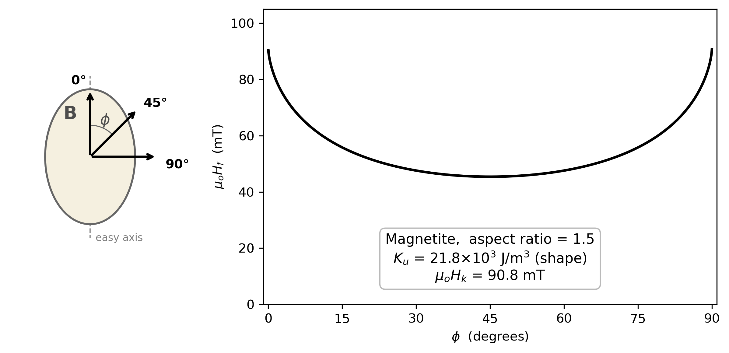
Figure 5.2:The flipping field required to irreversibly switch the magnetization vector from one easy direction to the other in a single domain particle dominated by uniaxial shape anisotropy (here calculated for a prolate magnetite spheroid with aspect ratio of 1.5). The angle is measured between the applied field and the easy axis direction opposite to . The minimum flipping field occurs at = 45°. At = 0° and 90°, equals the microscopic coercivity = 2/. Note that the magnetization reversal at = 90° is entirely reversible — the moment deflects toward the applied field but returns to its original easy axis direction when the field is removed, so no remanence in the applied direction is acquired.
The flipping condition depends not only on the applied field magnitude but also on the direction that it makes with the easy axis (see versus in Figure 5.2). When is parallel to the easy axis (zero) (and anti-parallel to ), is 58 mT as we found before. drops steadily as the angle between the field and the easy axis increases until an angle of 45° when starts to increase again. According to Equation 5.6, is undefined when = 90°, so when the field is applied at right angles to the easy axis, there is no field sufficient to flip the moment.
5.2Hysteresis loops
In this section, we will develop the theory for predicting the response of substances to the application of external fields in experiments that generate hysteresis loops. Hysteresis loops result from measurements of magnetic moment as a function of applied field . In a standard experiment, the field is ramped to a high field with the goal of saturating a specimen (e.g. 1.5 T) and then cycled to the opposite field direction and back up to the positive. The response of a specimen can give insight into mineralogy, domain state, and grain size. These experiments are typically made on a vibrating sample magnetometer (VSM) where a specimen is mounted on a thin rod between the pole pieces of an electromagnet that supplies the applied field . The specimen is vibrated mechanically (typically via a piezoelectric or linear motor drive) at a known frequency and amplitude. This vibration causes a changing magnetic flux through nearby pickup coils, inducing a voltage proportional to the magnetic moment of the specimen. A lock-in amplifier extracts the signal at the drive frequency, providing high-sensitivity measurements of measured as a function of applied field .
Let us begin by considering what happens to single particles when subjected to applied fields in the cycle known as the hysteresis loop. From the last section, we know that when a single domain, uniaxial particle is subjected to an increasing magnetic field the magnetization is gradually drawn into the direction of the applied field. If the flipping condition is not met, then the magnetization will return to the original direction when the magnetic field is removed. If the flipping condition is met, then the magnetization undergoes an irreversible change and will be in the opposite direction when the magnetic field is removed.
5.2.1Uniaxial anisotropy
Imagine a single domain particle with uniaxial anisotropy. Because the particle is single domain, the magnetization is at saturation and, in the absence of an applied field, is constrained to lie along the easy axis. Now suppose we apply a magnetic field in the opposite direction (see track #1 in Figure 5.3a). When reaches in magnitude, the magnetization flips to the opposite direction (track #2 in Figure 5.3) and will not change further regardless of how high the field goes. The field then is decreased to zero and then increased along track #3 in Figure 5.3 until is reached again. The magnetization then flips back to the original direction (track #4 in Figure 5.3a).
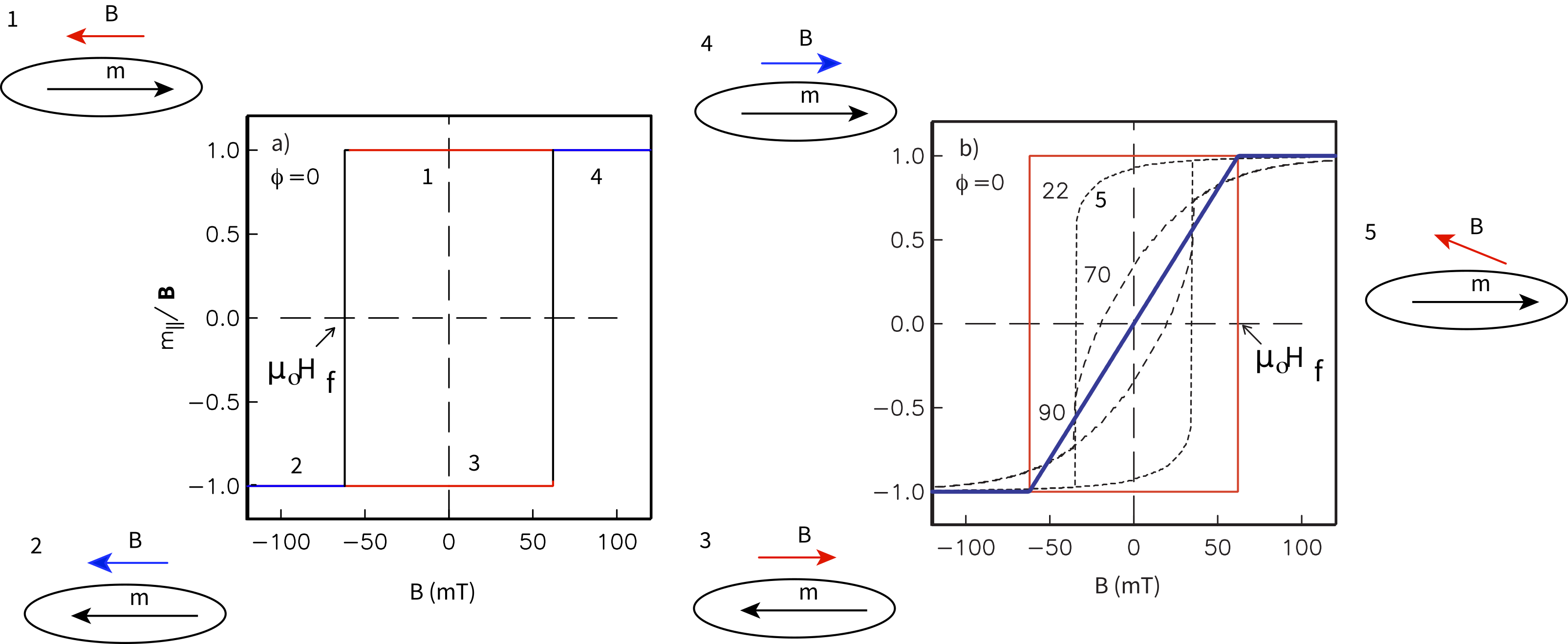
Figure 5.3:a) Moment measured for the particle () with applied field starting at 0 mT and increasing in the opposite direction along track #1. When the flipping field is reached, the moment switches to the other direction along track #2. The field then switches sign and decreases along track #3 to zero, then increases again to the flipping field. The moment flips and the field increases along track #4. b) The component of magnetization parallel to +B versus for field applied with various angles .
Applying fields at arbitrary angles to the easy axis results in loops of various shapes (see Figure 5.3b). As approaches 90°, the loops become thinner. Remember that the flipping fields for = 22° and are similar (see Figure 5.2) and are lower than that when , but the flipping field for is infinite, so that “loop” is closed and completely reversible.
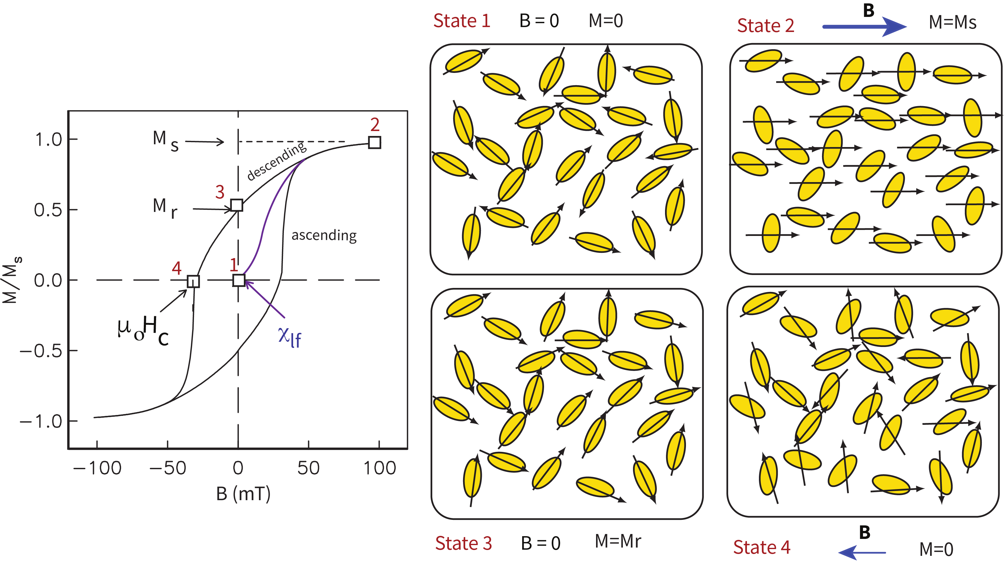
Figure 5.4:Net response of a random assemblage of uniaxial single domain particles. Snapshots of magnetization states (squares labeled 1 to 4) for representative particles are shown in the panels labeled State 1–4. The initial demagnetized state is “State 1” with no applied field and zero net magnetization. The initial slope as the field is increased from zero is the low-field susceptibility . When all the moments are parallel to the applied field (State 2), the magnetization is at saturation . When the field is returned to zero, the magnetization is the remanent magnetization (; State 3). When the field is applied in the opposite direction and has flipped half the moments (State 4), the net magnetization is zero and the field is the bulk coercive field .
In rocks with an assemblage of randomly oriented particles with uniaxial anisotropy, we would measure the sum of all the millions of tiny individual loops. A specimen from such a rock would yield a loop similar to that shown in Figure 5.4a. If the field is first applied to a demagnetized specimen, the initial slope is the (low field) magnetic susceptibility () first introduced in Chapter 1. From the treatment in Section 5.1 it is possible to derive the equation for this initial (ferromagnetic) susceptibility (for more, see O'Reilly (1984)).
If the field is increased beyond the flipping field of some of the magnetic grains and returned to zero, the net remanence is called an isothermal remanent magnetization (IRM). If the field is increased to , all the magnetizations are drawn into the field direction and the net magnetization is equal to the sum of all the individual magnetizations and is the saturation magnetization . When the field is reduced to zero, the moments relax back to their individual easy axes, many of which are at a high angle to the direction of the saturating field and cancel each other out with the net remanence after saturation is termed the saturation remanent magnetization (and sometimes the saturation isothermal remanence sIRM). The field necessary in the opposing direction to reduce the net moment from the to zero is defined as the coercive field () (or coercivity).
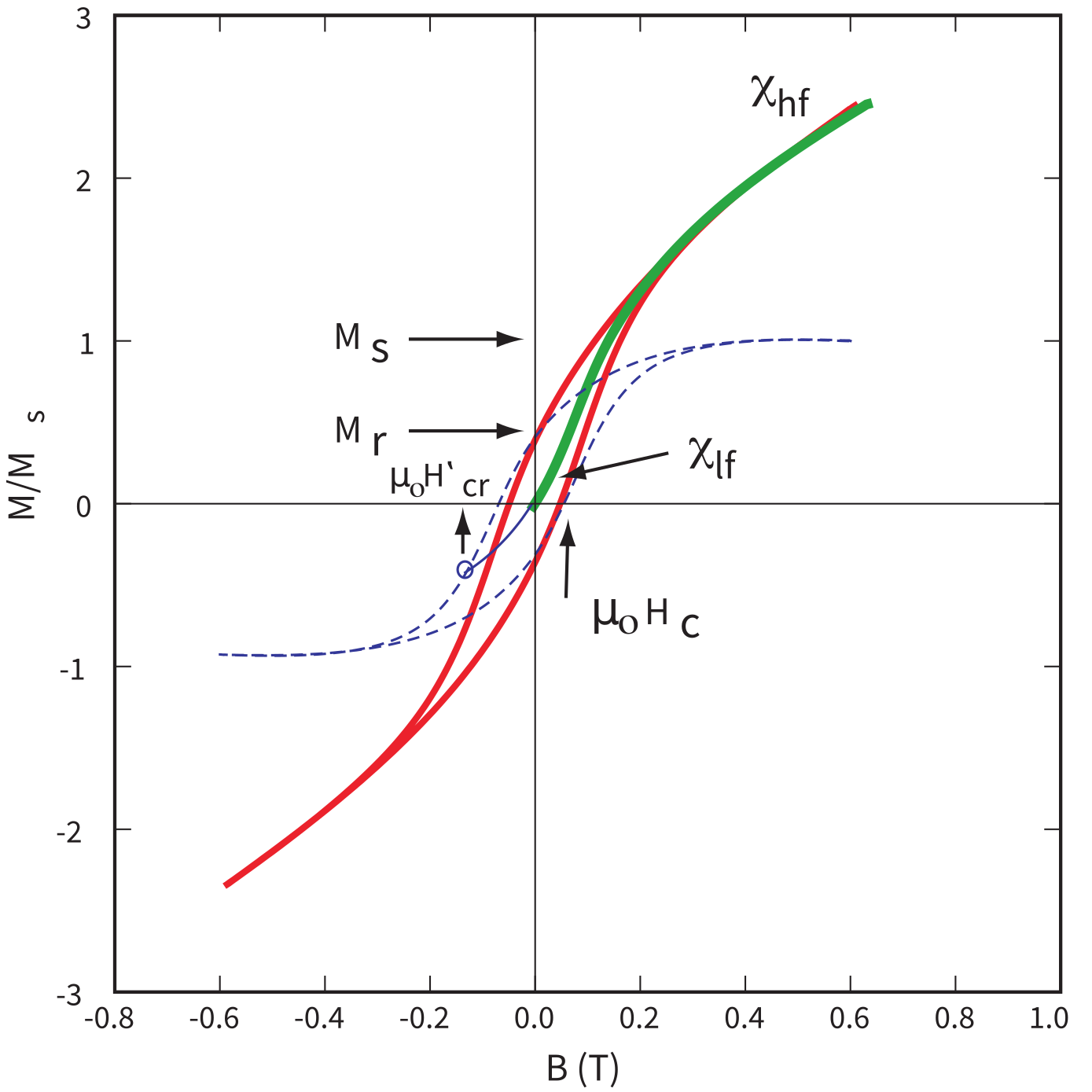
Figure 5.5:Heavy green line: initial behavior of demagnetized specimen as applied field ramps up from zero field to a saturating field. The initial slope is the initial or low-field susceptibility . After saturation is achieved the slope is the high-field susceptibility which is the non-ferromagnetic contribution, in this case the paramagnetic susceptibility (because is positive.) The dashed blue line is the hysteresis loop after the paramagnetic slope has been subtracted. Saturation magnetization is the maximum value of magnetization after slope correction. Saturation remanence is the value of the magnetization remaining in zero applied field. Coercivity () and coercivity of remanence are as in Figure 5.4a. A loop that does not achieve a saturating field (red in Figure 5.4a) is called a minor hysteresis loop, while one that does is called the outer loop.
For a random assemblage of single domain uniaxial particles, = 0.5. In the case of equant grains of magnetite for which magnetocrystalline anisotropy dominates, there are four easy axes, instead of two as in the uniaxial case (see Chapter 4). The maximum angle between an easy axis and an applied field direction is 55°. As a result of these additional easy axes, the remanent magnetization with be closer to the applied field direction when the field is removed. A random assemblage of particles with cubic anisotropy will therefore have a much higher saturation remanence () with a theoretical ratio of of 0.87, as opposed to 0.5 for the uniaxial case Joffe & Heuberger (1974).
The coercivity of remanence is defined as the magnetic field required to reduce the net remanence to zero after saturation. In other words, if a specimen is first given a saturation remanence and then subjected to an increasingly strong field in the opposite direction, is the backfield at which the remanence passes through zero.
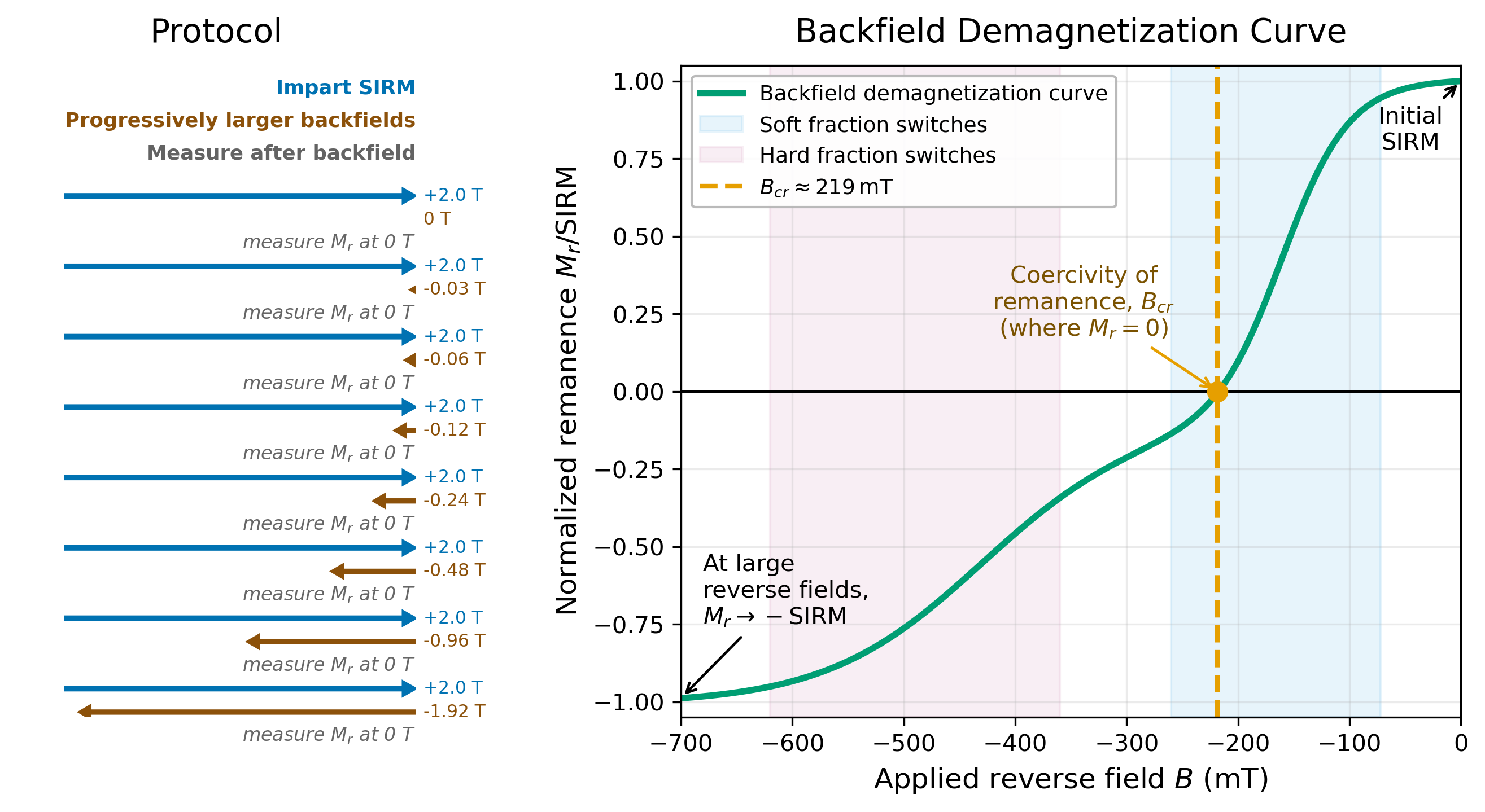
Figure 5.6:Schematic of a backfield demagnetization experiment. (Left) The measurement protocol begins by imparting a saturation isothermal remanent magnetization (SIRM) in a strong positive field (here +2.0 T, blue arrows). A smaller reverse field is then applied (brown arrows) and removed, and the remanent magnetization is measured in zero field. This cycle of re-saturating, applying a progressively larger reverse field, and measuring is repeated. (Right) The resulting backfield demagnetization curve plots the normalized remanence /SIRM against the applied reverse field . The curve begins at +1 (full SIRM) and decreases monotonically toward -1 (SIRM) as increasingly large reverse fields switch the magnetization of progressively higher-coercivity grain populations. The field at which defines the coercivity of remanence, (dashed orange line), a bulk measure of the sample’s resistance to demagnetization. In this two-component example, a soft fraction (blue shading) switches at relatively low reverse fields, while a hard fraction (pink shading) requires substantially larger fields with the two inflections characteristic of a mixed coercivity assemblage.
The most direct way to measure coercivity of remanence is the backfield experiment. After saturating a specimen in a strong positive field and returning the field to zero (establishing ), one applies a field in the negative direction, increasing its magnitude in steps. At each step, the field is briefly removed and the remanence is measured. The resulting curve (Figure 5.6) starts at and decreases monotonically. The field at which the remanence crosses zero is (or equivalently ). The backfield curve contains more information than this single parameter — its derivative with respect to the applied field gives the coercivity spectrum, which represents the distribution of switching fields within the grain assemblage. This distribution can be analyzed through coercivity unmixing techniques to identify distinct magnetic components within a specimen (see Chapter 6).
5.2.2Magnetic susceptibility
Figure 5.4a is the loop created in the idealized case in which only uniaxial ferromagnetic particles participated in the hysteresis measurements; in fact the curve is entirely theoretical. In “real” specimens there can be paramagnetic, diamagnetic AND ferromagnetic particles and the loop may well look like that shown in Figure 5.5. The initial slope of a hysteresis experiment starting from a demagnetized state in which the field is ramped from zero up to higher values is the low field magnetic susceptibility or (see Figure 5.5). If the field is then turned off, the magnetization will return again to zero. But as the field increases past the lowest flipping field, the remanence will no longer be zero but some isothermal remanence. Once all particle moments have flipped and saturation magnetization has been achieved, the slope relating magnetization and applied field reflects only the non-ferromagnetic (paramagnetic and/or diamagnetic) susceptibility, here called high field susceptibility, . In order to estimate the saturation magnetization and the saturation remanence, we must first subtract the high field slope. So doing gives us the blue dashed line in Figure 5.5 from which we may read the various hysteresis parameters illustrated in Figure 5.4b.
5.2.3Superparamagnetic particles
In superparamagnetic (SP) particles, the total magnetic energy (where is the total energy density from Equation 5.3 and is the particle volume) is balanced by thermal energy (where is Boltzmann’s constant and is the absolute temperature). This behavior can be modeled using statistical mechanics in a manner similar to that derived for paramagnetic grains in Chapter 3. A reasonable approximation is the Langevin function,
where is the magnetization, is the saturation magnetization, and is the number of particles of volume . The argument is the ratio of magnetostatic to thermal energy, with the applied magnetic field (the remaining variables as defined above). Equation 5.7 is the familiar Langevin function from our discussion of paramagnetic behavior (see Chapter 3); hence the term “superparamagnetic” for such particles.
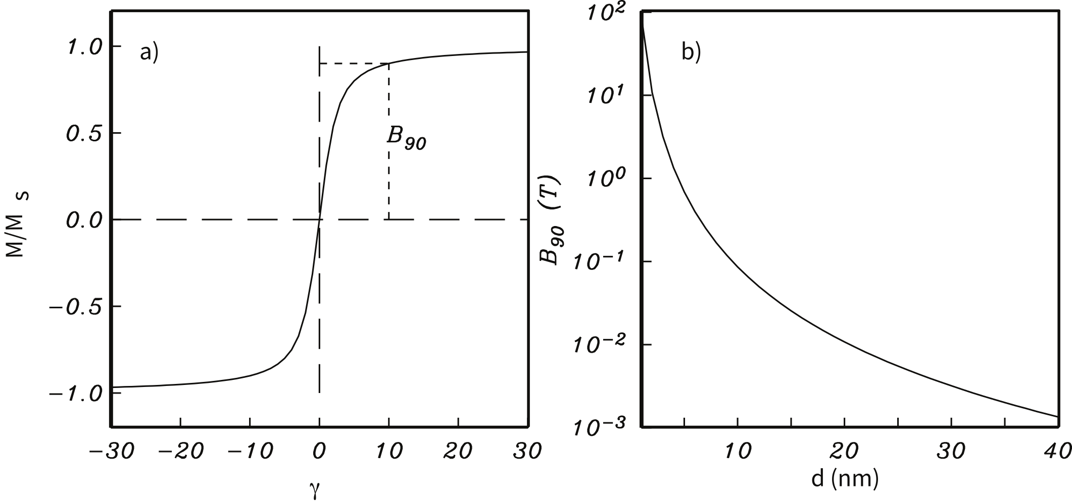
Figure 5.7:a) The contribution of SP particles with saturation magnetization and cubic edge length . . There is no hysteresis. b) The field at which the magnetization reaches 90% of the maximum is when . [Figure from Tauxe et al. (1996).]
The contribution of SP particles for which the Langevin function is valid for given values of and is shown in Figure 5.7a. The field at which the population reaches 90% saturation occurs at . Assuming particles of magnetite ( = 480 kAm) and room temperature ( K), can be evaluated as a function of (see Figure 5.7b). Because of its inverse cubic dependence on , rises sharply with decreasing and is hundreds of tesla for particles a few nanometers in size, approaching paramagnetic values. is a quick guide to the SP slope (the SP susceptibility ) contributing to the hysteresis response and was used by Tauxe et al. (1996) as a means of explaining distorted loops sometimes observed for populations of SD/SP mixtures. (and ) is very sensitive to particle size with very steep slopes for the particles at the SP/SD threshold. The exact threshold size is still rather controversial, but Tauxe et al. (1996) argue that it is ~20 nm.
For low magnetic fields, the Langevin function can be approximated as . So we have:
If we substitute for (where is the permeability of free space and is the magnetic field strength) and rearrange this equation, we can get the superparamagnetic susceptibility as:
We can rearrange Equation 4.18 in Chapter 4 to solve for the volume at which a uniaxial grain passes through the superparamagnetic threshold:
where is the uniaxial anisotropy constant, is the relaxation time, and is the frequency factor (see Chapter 4).
Finally, we can substitute this volume into Equation 5.9 as the maximum volume of an SP grain, giving us:
Comparing this expression with that derived for ferromagnetic susceptibility in Section 5.2.1, we find that is a factor of larger than the equivalent single domain particle.
5.2.4Particles with domain walls
Moving domain walls around is much easier than flipping the magnetization of an entire particle coherently. The reason for this is the same as the reason that it is easier to move a rug by lifting up a small wrinkle and pushing that through the rug, than to drag the whole rug by the same amount. Because of the greater ease of changing magnetic moments in multidomain (MD) grains, they have lower coercive fields and saturation remanence is also much lower than for uniformly magnetized particles (see typical MD hysteresis loop in Figure 5.8a.)
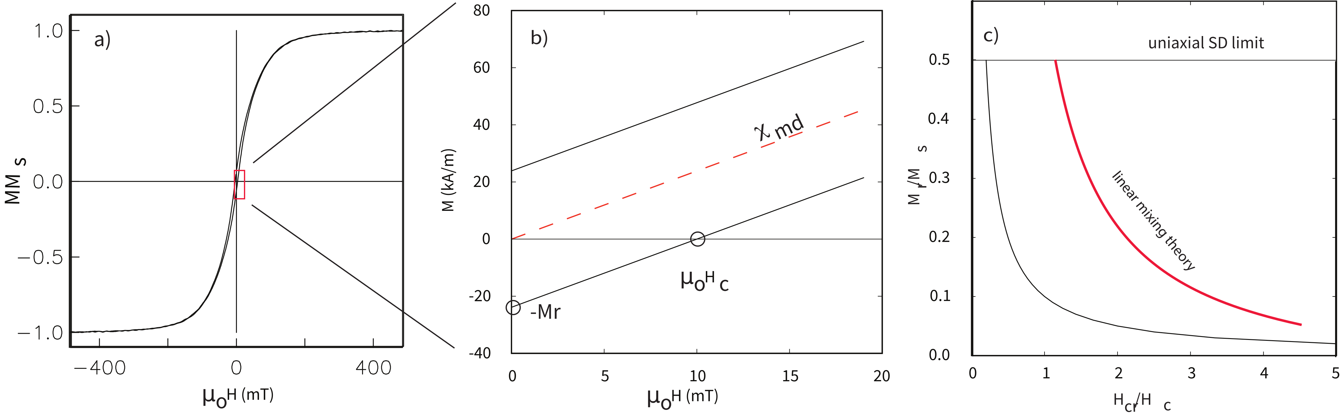
Figure 5.8:a) Typical hysteresis loop from a multidomain assemblage. b) Theoretical behavior for the region in the inset to a). c) Theoretical relationship between and for constant . Heavy red line is the theoretical linear mixing curve of SD/MD end-members. (See text.)
The key to understanding multidomain hysteresis is the reduction in multidomain magnetic susceptibility from “true” magnetic susceptibility () because of self-demagnetization. The true susceptibility would be that obtained by measuring the magnetic response of a particle to the internal field (applied field minus the demagnetizing field — see Section 4.1.5; see Dunlop, 2002a Dunlop (2002)). Recalling that the demagnetizing factor is , the so-called screening factor is and . If we assume that is linear for fields less than the coercivity, then by definition (see Figure 5.8b). From this, we get:
In the case of multidomain susceptibility, is much larger than and .
By a similar argument, coercivity of remanence () is suppressed by the screening factor which gives coercivity so:
from which we get the ratio:
Putting all this together leads us to the remarkable relationship noted by Day et al. (1977) (see also Dunlop (2002)):
When is constant, Equation 5.15 is a hyperbola. For a single mineralogy, we can expect to be constant, but depends on grain size and the state of stress which are unlikely to be constant for any natural population of magnetic grains. Dunlop (2002a) Dunlop (2002) argues that if the main control on susceptibility and coercivity is domain wall motion through a terrain of variable wall energies, then and would be inversely related and gives a tentative theoretical value for in magnetite of about 45 kAm. This, combined with the value of for magnetite of 480 kAm gives a value for . When anchored by the theoretical maximum for uniaxial single domain ratio of , we get the curve shown in Figure 5.8c. The major control on coercivity is grain size, so the trend from the SD limit down toward low ratios is increasing grain size.
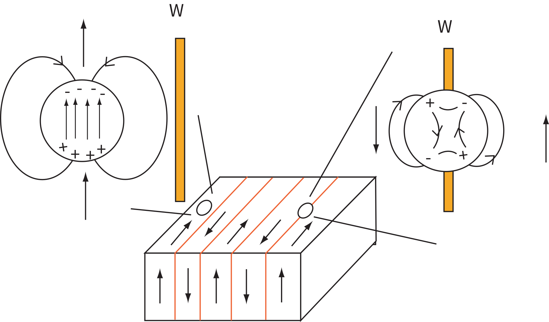
Figure 5.9:Interaction of a domain wall and a void. When the void is within a domain, free poles create a magnetic field which creates a self energy (Chapter 4). When a domain wall intersects the void, the self-energy is reduced. There are no exchange or magnetocrystalline anisotropy energy terms within the void, so the wall energy is reduced.
There are several possible causes of variability in wall energy within a magnetic grain, for example, voids, lattice dislocations, stress, etc. The effect of voids is perhaps the easiest to visualize, so we will consider voids as an example of why wall energy varies as a function of position within the grain. We show a particle with lamellar domain structure and several voids in Figure 5.9. When the void occurs within a uniformly magnetized domain (left of figure), the void sets up a demagnetizing field as a result of the free poles on the surface of the void. There is therefore, a self-energy associated with the void. When the void is traversed by a wall, the free pole area is reduced, reducing the demagnetizing field and the associated self-energy. Therefore, the energy of the void is reduced by having a wall bisect it. Furthermore, the energy of the wall is also reduced, because the area of the wall in which magnetization vectors are tormented by exchange and magnetocrystalline energies is reduced. The wall gets a “free” spot if it bisects a void. The wall energy therefore is lower as a result of the void.
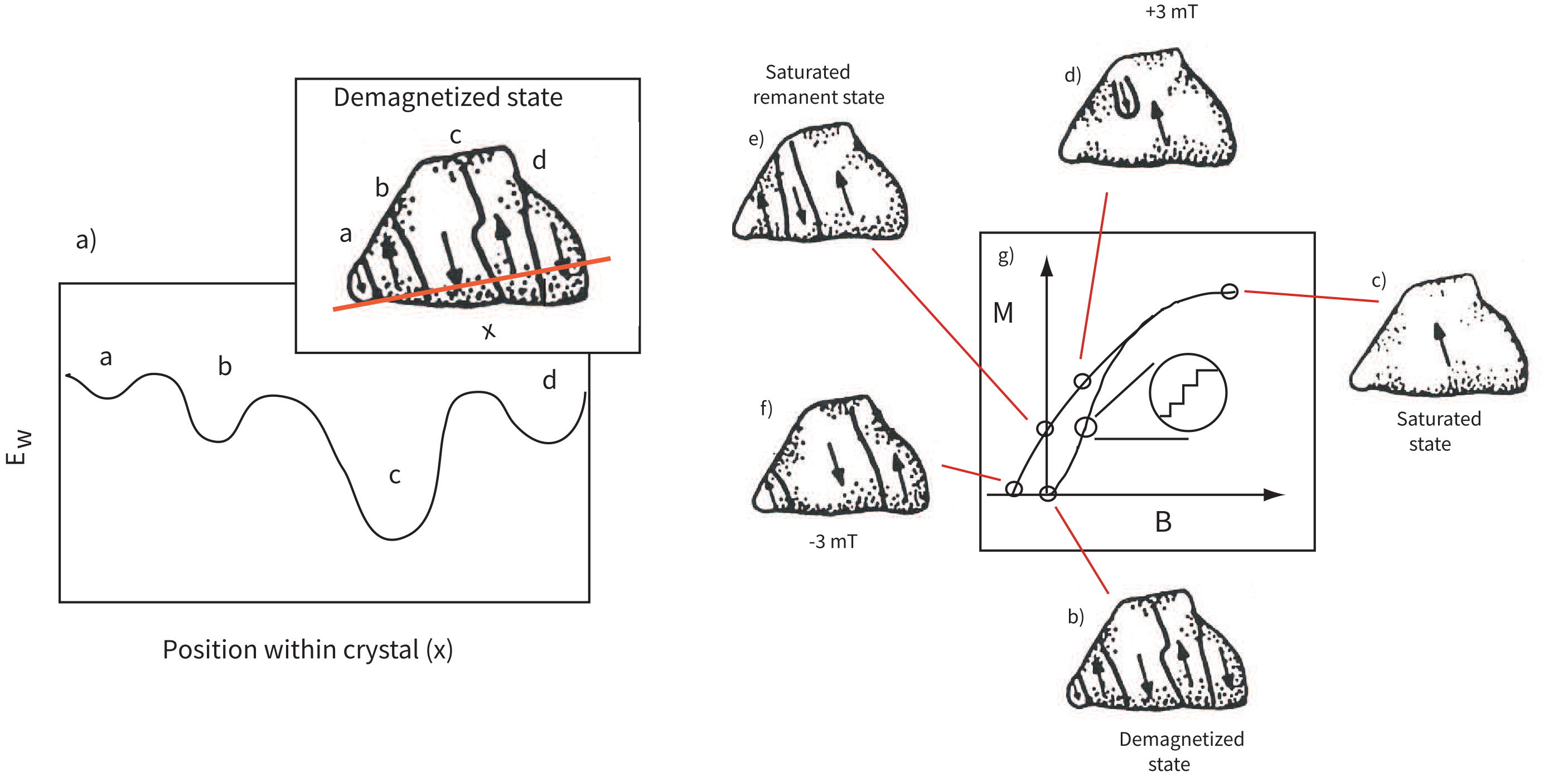
Figure 5.10:a) Schematic view of wall energy across a transect of a multidomain grain. Inset: Placement of domain walls in the demagnetized state. [Domain observations from Halgedahl & Fuller (1983).] b–g) Schematic view of the magnetization process in MD grain shown in previous figure. b) Demagnetized state, c) in the presence of a saturating field, d) field lowered to +3 mT, e) remanent state, f) backfield of −3 mT, g) resulting loop. Inset shows detail of domain walls moving by small increments called Barkhausen jumps. [Domain wall observations from Halgedahl & Fuller (1983); schematic loop after O'Reilly (1984).]
In Figure 5.10, we show a sketch of a hypothetical transect of across a particle. There are four LEMs labelled a–d. Domain walls will distribute themselves throughout the grain in order to minimize the net magnetization of the grain and also to try to take advantage of LEMs in wall energy.
Domain walls move in response to external magnetic fields (see Figure 5.10b–g). Starting in the demagnetized state (Figure 5.10b), we apply a magnetic field that increases to saturation (Figure 5.10c). As the field increases, the domain walls move in sudden jerks as each successive local wall energy high is overcome. This process, known as Barkhausen jumps, leads to the stair-step like increases in magnetization (shown in the inset of Figure 5.10g). At saturation, all the walls have been flushed out of the crystal and it is uniformly magnetized. When the field decreases again, to say +3 mT (Figure 5.10d), domain walls begin to nucleate, but because the energy of nucleation is larger than the energy of denucleation, the grain is not as effective in cancelling out the net magnetization, hence there is a net saturation remanence (Figure 5.10e). The walls migrate around as a magnetic field is applied in the opposite direction (Figure 5.10f) until there is no net magnetization. The difference in nucleation and denucleation energies was called on by Halgedahl & Fuller (1983) to explain the high stability observed in some large magnetic grains.
5.3Hysteresis of mixtures of SP, SD and MD grains
Day et al. (1977) popularized the use of diagrams like that shown in Figure 5.8c which are known as Day diagrams. They placed quasi-theoretical bounds on the plot whereby points with ratios above 0.5 were labelled single domain (SD), and points falling in the box bounded by and were labelled pseudo-single domain (PSD). Points with below 0.05 were labelled multidomain (MD). This paper has been cited over 800 times in the literature and the Day plot still serves as the principal way that rock and paleomagnetists determine domain state and grain size.
The problem with the Day diagram is that virtually all paleomagnetically useful specimens yield hysteresis ratios that fall within the PSD box. In the early 90s, paleomagnetists began to realize that many things besides the trend from SD to MD behavior control where points fall on the Day diagram. Pick & Tauxe (1994) pointed out that mixtures of SP and SD grains would have reduced ratios and enhanced ratios. Tauxe et al. (1996) modelled distributions of SP/SD particles and showed that the SP-SD trends always fall above those observed from MD particles (modelled in Figure 5.8c).
Dunlop (2002) argued that because for SP grains is zero, the suppression of the ratio is directly proportional to the volume fraction of the SP particles. Moreover, coercivity of remanence remains unchanged, as it is entirely due to the non-SP fraction. Deriving the relationship of coercivity, however, is not so simple. It depends on the superparamagnetic susceptibility (), which in turn depends on the size of the particle and also the applied field (see Section 5.2.3). In his simplified approach, Dunlop could only use a single (small) grain size, whereas in natural samples, there will always be a distribution of grain sizes. It is also important to remember that volume goes as the cube of the radius and for a mixture to display any SP suppression of almost all of the particles must be SP. It is impossible that these would all be of a single radius (say 10 or 15 nm); there must be a distribution of sizes. Moreover, Dunlop (2002) neglected the complication in SP behavior as the particles reach the SD threshold size, whereas it is expected that many (if not most) natural samples containing both SP and SD grain sizes will have a large volume fraction of the largest SP sizes, making their neglect problematic.
Hysteresis ratios of mixtures of SD and MD particles will also plot in the “PSD” box. Dunlop (2002) derived the theoretical behavior of such mixtures on the Day diagram. The key equations are 1) Equation 9 from Dunlop (2002) which governs the behavior of the ratio as a function of the volume fraction of single domain material () and multidomain material ():
Equation 10 from Dunlop (2002) which governs the behavior of coercivity:
and 3) Equation 11 from Dunlop (2002) which governs the behavior of coercivity of remanence in SD/MD mixtures:
where and are the susceptibilities of the SD and MD fractions respectively and and are the vs slopes of the SD and MD remanences respectively. What we need to calculate the SD/MD mixing curve are values for the various parameters for single domain and multi domain end-members. These were measured empirically for the MV1H bacterial magnetosomes (see Chapter 6) and commercial magnetite (041183 of Wright Company) by Dunlop & Carter-Stiglitz (2006) and shown in the table below.
| SD/MD | (A mT) | (MA mT) | (mT) | (mT) | |
|---|---|---|---|---|---|
| SD | 0.5 | 5.2 | 4.55 | 46 | 52.5 |
| MD | 0.02 | 4.14 | 0.88 | 5.56 | 26.1 |
: Empirical values for hysteresis parameters measured for single domain (SD) and multidomain (MD) end-members of Dunlop & Carter-Stiglitz (2006).
Using the linear mixing model of Dunlop (2002), we plot the theoretical mixing curve predicted for these empirically constrained end-members as the heavy red line in Figure 5.8c.
If a population of SD particles are so closely packed as to influence one another, there will be an effect of particle interaction. This will also tend to suppress the ratio, drawing the hysteresis ratios down into the PSD box. Finally, the PSD box could be populated by pseudo-single domain grains themselves. Here we will dwell for a moment on the meaning of the term “pseudo-single domain”, which has evolved from the original meaning posed by Stacey (1961) (see discussion in Tauxe et al. (2002)). In an attempt to explain trends in TRM acquisition Stacey envisioned that irregular shapes caused unequal domain sizes, which would give rise to a net moment that was less than the single domain value, but considerably higher than the very low efficiency expected for large MD grains. The modern interpretation of PSD behavior is complicated micromagnetic structures that form between classic SD (uniformly magnetized grains) and MD (domain walls) such as the flower or vortex remanent states (see, e.g., Figure 4.5 in Chapter 4). Taking all these factors into account means that interpretation of the Day diagram is far from unique. The simple calculations of Dunlop (2002) are likely to be inappropriate for almost all natural samples.
5.4First order reversal curves
Hysteresis loops can yield a tremendous amount of information yet much of this is lost by simply estimating the set of summary parameters , etc. Mayergoyz (1986) developed a method using what are known as First Order Reversal Curves or FORCs to represent hysteresis data. In the FORC experiment, a specimen is subjected to a saturating field, as in most hysteresis experiments. The field is lowered to some field (starting with small changes from the saturating field), then increased again to saturation (see Figure 5.11a). The magnetization curve between and is a “FORC”. A series of FORCs (see Figure 5.11b) can be generated to the desired resolution to fill the interior of the major outside loop with these minor loops.
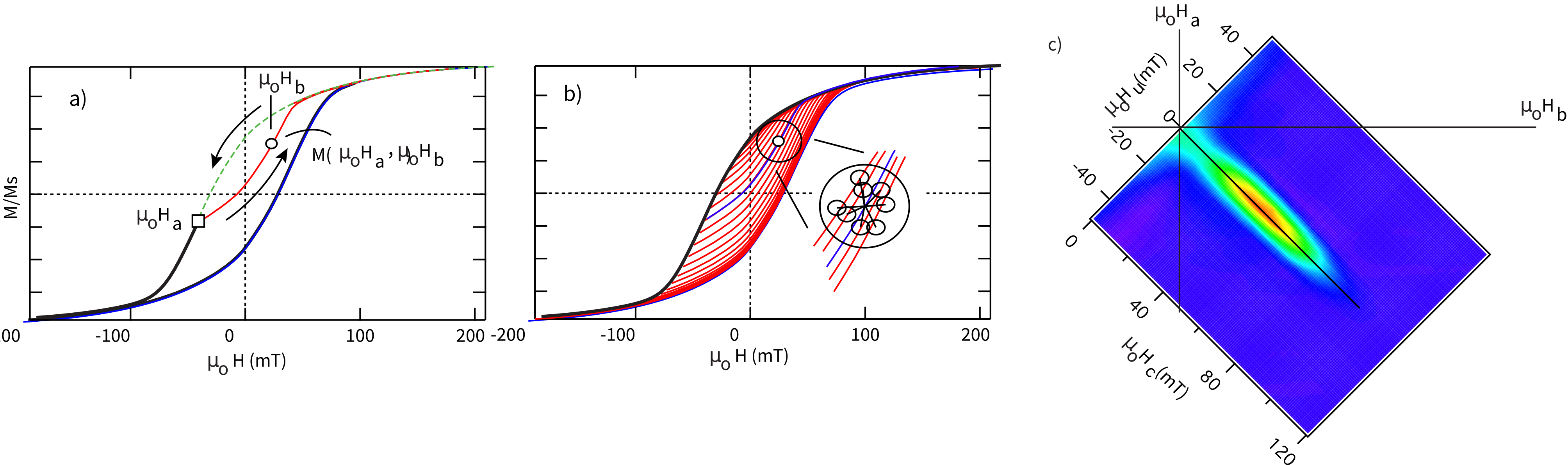
Figure 5.11:a) Dashed line is the descending magnetization curve taken from a saturating field to some field . Red line is the first order reversal curve (FORC) from returning to saturation. At any field there is a value for the magnetization . b) A series of FORCs for a single domain assemblage of particles. At any point there are a set of related “nearest neighbor” measurements (circles in inset) that can be used to develop a FORC diagram using smoothing algorithms. c) A contour plot of the FORC density surface for data in b). Specimen is of the Tiva Canyon Tuff, courtesy of the Institute for Rock Magnetism.
To transform FORC data into a useful form for interpretation, the measured magnetization at each point on the FORC diagram is fit with a second-order polynomial of the form
where the are fitted coefficients determined from neighboring measurement points (e.g., those within the circle shown in Figure 5.11b). The coefficient is the FORC density at that point (Pike et al. (1999); Roberts et al. (2000)). The choice of how many neighbors to include and how to weight them constitutes the smoothing of the FORC diagram, and various approaches have been developed, including the VARIFORC method of Egli (2013) which allows the degree of smoothing to vary across the diagram. A FORC diagram is the contour plot of the FORC densities, rotated such that and .
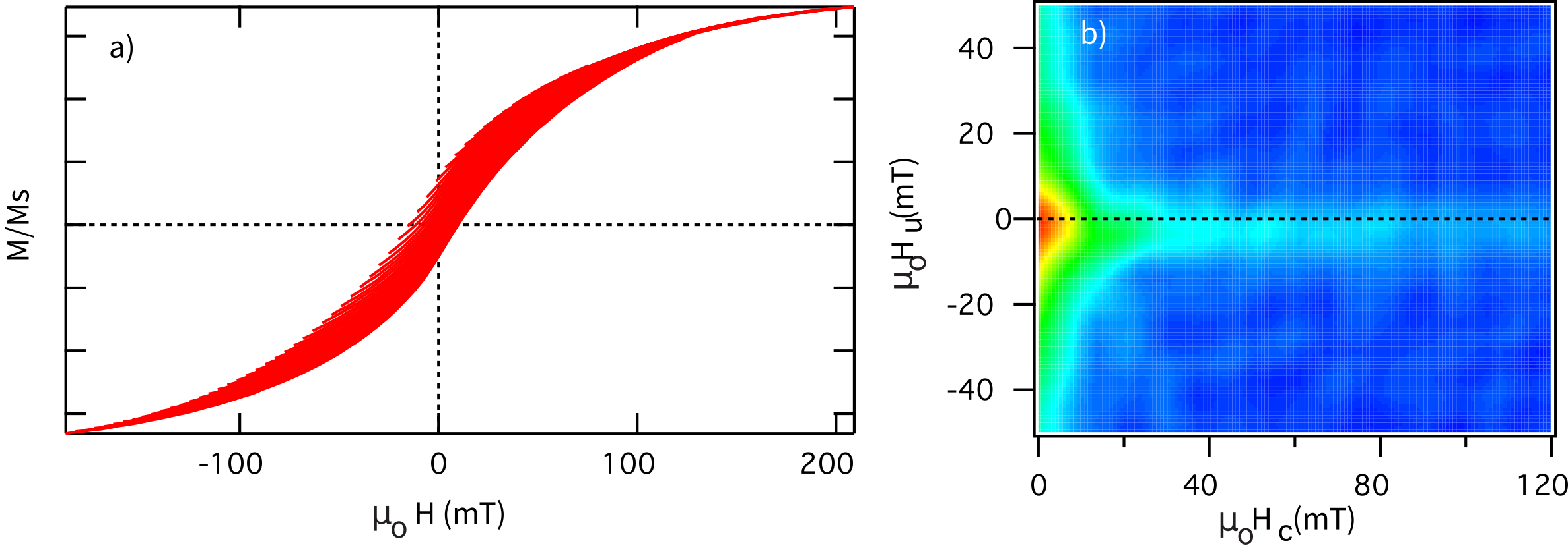
Figure 5.12:a) A series of FORCs for a specimen from the Stillwater Layered Intrusion. b) FORC diagram for data in a). Data are courtesy of J.S. Gee.
Imagine we travel down the descending magnetization curve (dashed line in Figure 5.11a) to a particular field less than the smallest flipping field in the assemblage. If the particles are single domain, the behavior is reversible and the first FORC will travel back up the descending curve. It is only when exceeds the flipping field of some of the particles that the FORC will trace a new curve on the inside of the hysteresis loop. In the simple single domain, non-interacting, uniaxial magnetite case, the FORC density in the quadrants where and are of the same sign must be zero. Indeed, FORC densities will only be non-zero for the range of flipping fields because these are the bounds of the flipping field distribution. So the diagram in Figure 5.11c is nearly that of an ideal uniaxial SD distribution. A hallmark of such non-interacting SD assemblages is the “central ridge”—a narrow, sharp ridge of FORC density along the axis at (Egli et al. (2010)). The central ridge arises because each SD grain flips irreversibly at a single coercivity and contributes density at that value with no vertical spread. When magnetostatic interactions are present among SD grains, the central ridge broadens vertically, so the width of the ridge along the axis can serve as a measure of interaction field strength (Egli et al. (2010); Zhao et al. (2017)).
Consider now the case in which a specimen has magnetic grains with non-uniform magnetizations such as vortex structures or domain walls. Unlike coherent SD reversal, these structures can change at fields well below the flipping field for coherent rotation. So while SD behavior is reversible if the field change doesn’t reach the flipping field, the magnetization curve may not be reversible for MD and vortex state grains. In vortex state grains, this irreversibility arises from the nucleation and annihilation of the vortex core—abrupt changes in the magnetization state that occur at different fields on the descending and ascending branches (Zhao et al. (2017); Lascu et al. (2018)). In multidomain grains, domain walls jump between local energy minima (from LEM to LEM) as the field changes, producing irreversibility through a series of small discrete steps. The resulting FORC for such behavior would have much of the “action” in the region where is positive. When transformed to and , the diagram will have high densities for small but over a range of . The example shown in Figure 5.12 is of a specimen that likely has grains in the vortex state. The FORC diagram in Figure 5.12b has some of the FORC densities concentrated along the axis characteristic of single domain specimens (e.g., Figure 5.11c), but there is also concentration along the axis characteristic of vortex state and multidomain specimens.
As a result, FORC diagrams can provide insight into domain state (Zhao et al. (2017); Lascu et al. (2018)). SD grains produce the central ridge described above, with the distribution along reflecting the coercivity spectrum of the assemblage. Vortex state grains generate a broad distribution that is spread vertically along the axis and shifted toward low , reflecting the range of fields over which vortex cores nucleate and annihilate. multidomain grains contribute FORC density concentrated near the origin at very low and low , consistent with the ease with which domain walls are displaced. Because natural specimens commonly contain mixtures of these grain populations, FORC diagrams often show superimposed contributions—for example, a central ridge from an SD fraction alongside a broader vortex state signal—allowing the relative contributions of different domain states to be assessed in ways that bulk hysteresis parameters alone cannot resolve.
Supplemental Reading: Dunlop & Özdemir (1997), chapters 5 and 11; O'Reilly (1984), pp 69–87; Dunlop (2002); Dunlop (2002).
5.5Problems
Problem 1
For a grain with uniaxial anisotropy in an external field, the direction of magnetization in this grain will be controlled entirely by the uniaxial anisotropy energy density and the magnetic interaction energy . The total energy can be written:
where is the angle of the applied field relative to the easy axis of magnetization and is the angle of the moment relative to the easy direction. Show that the flipping field of a grain whose moment is initially antiparallel to the field, i.e. = 180°, is given by:
Problem 2 [From Jeff Gee]
In this problem, we will begin to use some real data. The data files used with this book are part of the PmagPy distribution, which you should have already downloaded and installed. [See Preface for instructions.]
The file hysteresis.txt in the Chapter_5 directory contains data for a single hysteresis loop. Note that the units are as measured: H (Oe), moment (emu) and it is fine to leave them in these units.
a) Read the data into a Pandas DataFrame. Determine the high field slope at Oe. Typically one calculates separate slopes for the +H data and -H data and averages these. A general least squares polynomial fit (numpy.polyfit) should do the trick.
b) Use the slope you determined to plot both the original hysteresis loop and the slope-corrected loop (i.e. removing the high field paramagnetic slope).
c) What is the ratio (saturation remanence/saturation magnetization) for this sample? The coercivity of remanence () for this sample was estimated at 264 Oe. Based on the and ratios, is this sample more likely to contain single domain or multidomain grains?
d) This small sample has a mass of 10.6 mg. Assuming the magnetic material is magnetite, estimate the mass fraction of magnetite (92 Am/kg; note 1 emu/gm is equivalent to 1 Am/kg).
- Stoner, E. C., & Wohlfarth, E. P. (1948). A mechanism of magnetic hysteresis in heterogeneous alloys. Philosophical Transactions of the Royal Society of London A, 240(826), 599–642. 10.1098/rsta.1948.0007
- O’Reilly, W. (1984). Rock and Mineral Magnetism. Blackie. 10.1007/978-1-4684-8468-7
- Joffe, I., & Heuberger, R. (1974). Hysteresis properties of distributions of cubic single-domain ferromagnetic particles. Philosophical Magazine, 29(5), 1051–1059. 10.1080/14786437408226590
- Tauxe, L., Mullender, T. A. T., & Pick, T. (1996). Potbellies, wasp-waists, and superparamagnetism in magnetic hysteresis. Journal of Geophysical Research: Solid Earth, 101(B1), 571–583. 10.1029/95JB03041
- Dunlop, D. J. (2002). Theory and application of the Day plot (Mrs/Mₚ versus Hcr/Hc) 1. Theoretical curves and tests using titanomagnetite data. Journal of Geophysical Research: Solid Earth, 107(B3), 2056. 10.1029/2001JB000486
- Day, R., Fuller, M., & Schmidt, V. A. (1977). Hysteresis properties of titanomagnetites: Grain-size and compositional dependence. Physics of the Earth and Planetary Interiors, 13(4), 260–267. 10.1016/0031-9201(77)90108-X
- Halgedahl, S., & Fuller, M. (1983). The dependence of magnetic domain structure upon magnetization state with emphasis upon nucleation as a mechanism for pseudo-single-domain behavior. Journal of Geophysical Research: Solid Earth, 88(B8), 6505–6522. 10.1029/JB088iB08p06505
- Pick, T., & Tauxe, L. (1994). Characteristics of magnetite in submarine basaltic glass. Geophysical Journal International, 119(1), 116–128. 10.1111/j.1365-246X.1994.tb00917.x
- Dunlop, D. J., & Carter-Stiglitz, B. (2006). Day plots of mixtures of superparamagnetic, single-domain, pseudo-single-domain, and multidomain magnetites. Journal of Geophysical Research: Solid Earth, 111(B12), B12S09. 10.1029/2006JB004499
- Stacey, F. D. (1961). Theory of the magnetic properties of igneous rocks in alternating fields. Philosophical Magazine, 6(70), 1241–1260. 10.1080/14786436108212179
- Tauxe, L., Bertram, H. N., & Seberino, C. (2002). Physical interpretation of hysteresis loops: Micromagnetic modeling of fine particle magnetite. Geochemistry, Geophysics, Geosystems, 3(10), 1055. 10.1029/2001GC000241
- Mayergoyz, I. D. (1986). Mathematical models of hysteresis. Physical Review Letters, 56(15), 1518–1521. 10.1103/PhysRevLett.56.1518
- Pike, C. R., Roberts, A. P., & Verosub, K. L. (1999). Characterizing interactions in fine magnetic particle systems using first order reversal curves. Journal of Applied Physics, 85(9), 6660–6667. 10.1063/1.370176
- Roberts, A. P., Pike, C. R., & Verosub, K. L. (2000). First-order reversal curve diagrams: A new tool for characterizing the magnetic properties of natural samples. Journal of Geophysical Research: Solid Earth, 105(B12), 28461–28475. 10.1029/2000JB900326
- Egli, R. (2013). VARIFORC: An optimized protocol for calculating non-regular first-order reversal curve (FORC) diagrams. Global and Planetary Change, 110, 302–320. 10.1016/j.gloplacha.2013.08.003