Apparent polar wander is a central concept in paleomagnetism that provides quantitative constraints on tectonic plate motion through time. Interpreting paleomagnetic directions measured at Earth’s surface in terms of a geomagnetic field dominated by a geocentric dipole led to the definition of an equivalent pole position, the virtual geomagnetic pole (VGP), introduced in Chapter 2. In Chapter 14, we mentioned that averages of a number of VGPs that are considered to “average out” secular variation are known as paleomagnetic poles. When these are plotted on a map, such paleomagnetic poles “wander” away from the spin axis with increasing age of the rock unit sampled (e.g., Hospers (1955); Irving (1958)).
As illustrated in Figure 16.1, the apparent wandering of the north pole could be interpreted in two ways: wandering of continents whose paleomagnetic directions reflect the changing orientations and distances to the (fixed) pole (Figure 16.1a), or alternatively, the pole itself could be wandering, as in Figure 16.1b, while the continent remains fixed.
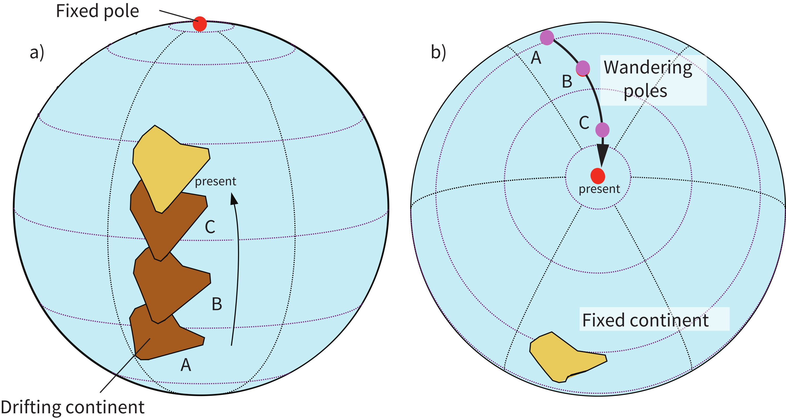
Figure 16.1:a) A moving continent will retain a record of changing paleomagnetic directions through time that reflect the changing orientations and distances to the pole (which is held fixed). The resulting path of observed pole positions is called an “apparent polar wander path” or APWP because in this case the pole is actually fixed and only appears to move when viewed from the continental frame of reference. b) On the other hand, if a continent is held fixed, the same changing paleomagnetic directions reflect the wandering of the pole itself. This is called “true polar wander” or TPW.
Data from a single continent cannot distinguish between these two hypotheses. Paleomagnetic data from multiple continents can, given our understanding that the time-averaged geomagnetic field is well approximated by a geocentric axial dipole. If the pole paths from two or more continents diverge back in time and there is a dipolar field (only one north pole), then it must be the continents that are doing the wandering. The initial discovery of divergent apparent polar wander paths between Europe and North America in the 1950s pointed towards the reality of continental drift that set the stage for the plate tectonic revolution Irving (1956). In this chapter, we will consider how apparent polar wander paths can be constructed and briefly discuss a few tectonic applications.
16.1Essentials of Plate Tectonic Theory
The rigid outer shell of the Earth, the lithosphere, is composed of many plates as shown in Figure 16.2. These plates are in constant motion with respect to one another, driven by convective flow in the underlying mantle and the gravitational pull of subducting slabs.
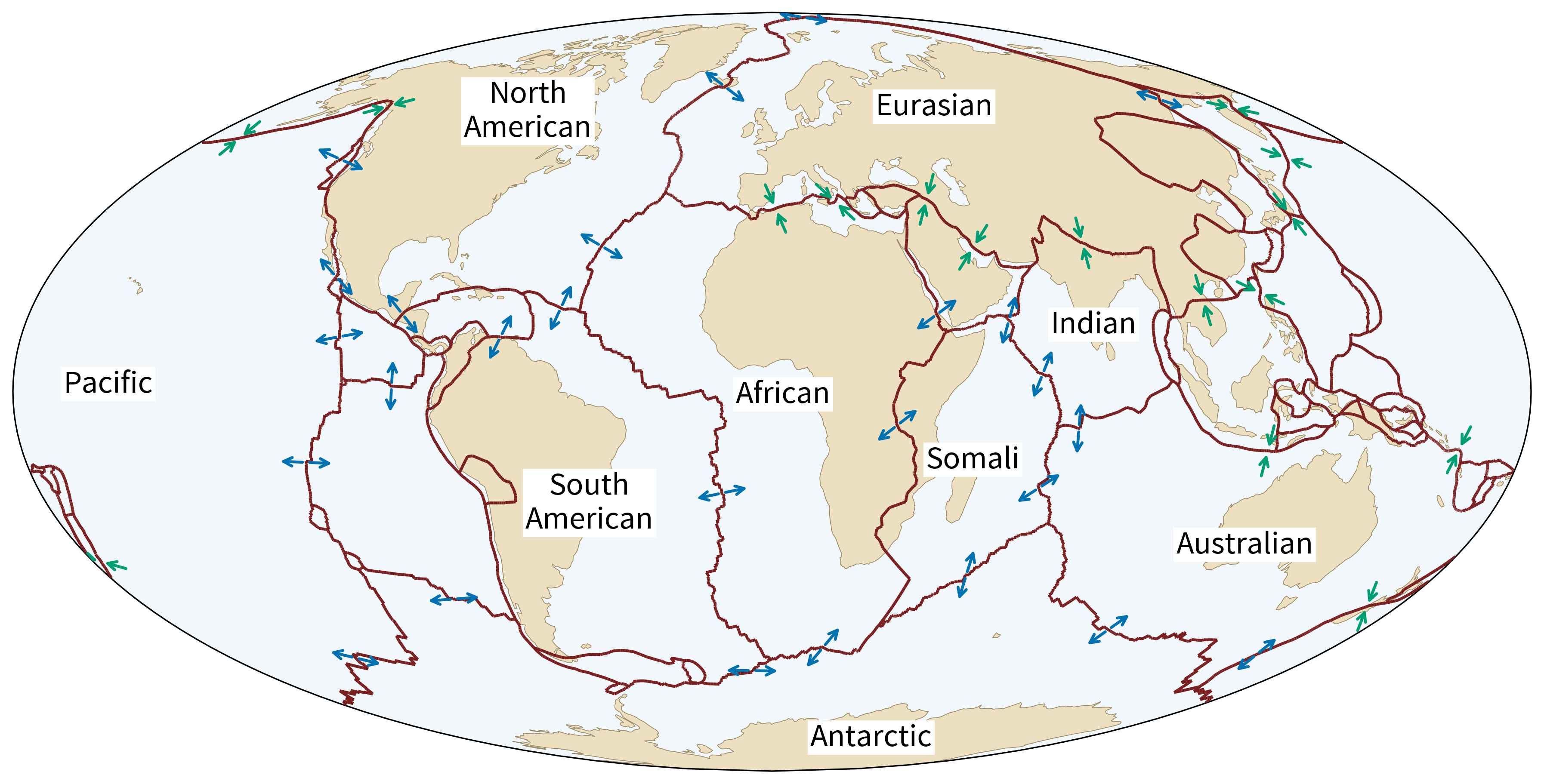
Figure 16.2:Major lithospheric plates with plate boundaries from the PB2002 model of Bird (2003). Blue arrows show the sense of divergent motion at oceanic spreading ridges; green arrows show convergent motion at subduction zones and continental collision boundaries.
The relative motion of two plates can be described by rotation about an Euler rotation vector, which is usually specified by a pole latitude/longitude on the surface of the Earth () and a rotation rate in °Myr. The velocity at a given point on a plate with respect to its “fixed” partner varies as a function of angular distance from the Euler pole () as:
where is the radius of the Earth as in Chapter 2. As an example, we show the motion of North America (NAM) with respect to “fixed” Europe (EUR) in Figure 16.3. The current NUVEL-1A Euler pole DeMets et al., 1994 is shown as the red circle. Lines of co-latitude correspond to in this projection, so the velocities (usually expressed in cm/yr; see red arrows in Figure 16.3) increase away from the pole, with a maximum at . Spreading rates can be determined from marine magnetic anomalies and their variation along the ridge crest can be fit with Equation 16.1 to determine the Euler pole position and rotation rate.
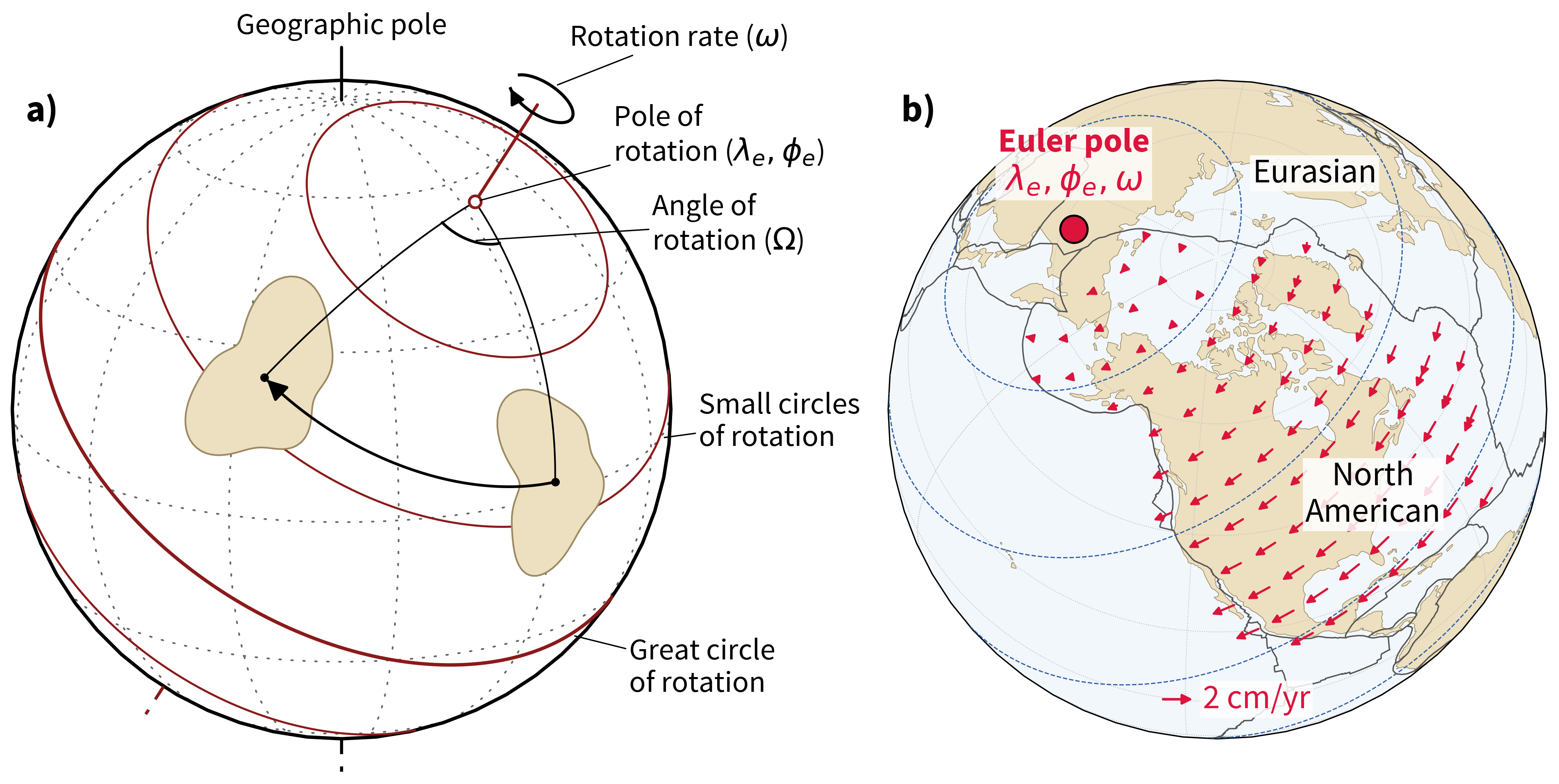
Figure 16.3:a) Euler’s theorem states that any rigid motion on a sphere can be represented as a rotation about an axis through Earth’s center. The surface trace of this axis defines the pole of rotation at (); a continent (tan) moves along a small circle of constant angular distance from this pole, sweeping through an angle of rotation at rate . b) Present-day motion of North America with respect to fixed Eurasia computed from the NUVEL-1A Euler pole DeMets et al., 1994 at (, ) = (62.4°N, 135.8°E) with = 0.21°/Myr. Red arrows show velocity vectors at grid points within the North American plate, with length proportional to speed (scale bar at bottom). Dashed blue lines are small circles of constant angular distance from the Euler pole at 30° intervals. Velocities increase with , reaching a maximum at .
An Euler pole describes the instantaneous rotation of one plate or continental fragment relative to another. For paleogeographic reconstruction, however, what is needed is the total rotation that restores a plate to a previous configuration (see Figure 16.6a). Such a rotation, defined by a pole and a specified rotation angle, is called a finite rotation pole. These can be found in several ways. Transforms and ridges define plate boundaries between two lithospheric plates and are to first order perpendicular and parallel to the direction of the finite rotation pole respectively. Marine magnetic anomalies can also be restored to the spreading centers via finite rotations. Also, a finite rotation can be found that restores a position defined for example by the continental margins (e.g., the Bullard fit of the Atlantic bordering continents, Bullard et al. (1965)) or that maximizes agreement of paleomagnetic poles after rotation. To illustrate what finite rotations accomplish, Figure 16.4 shows a paleogeographic reconstruction using the CEED6 plate model of Torsvik & Cocks (2017). The present-day configuration of continents is shown alongside their positions at 200 Ma, when North America and Europe were joined as part of the supercontinent Pangea, prior to the opening of the Atlantic Ocean.
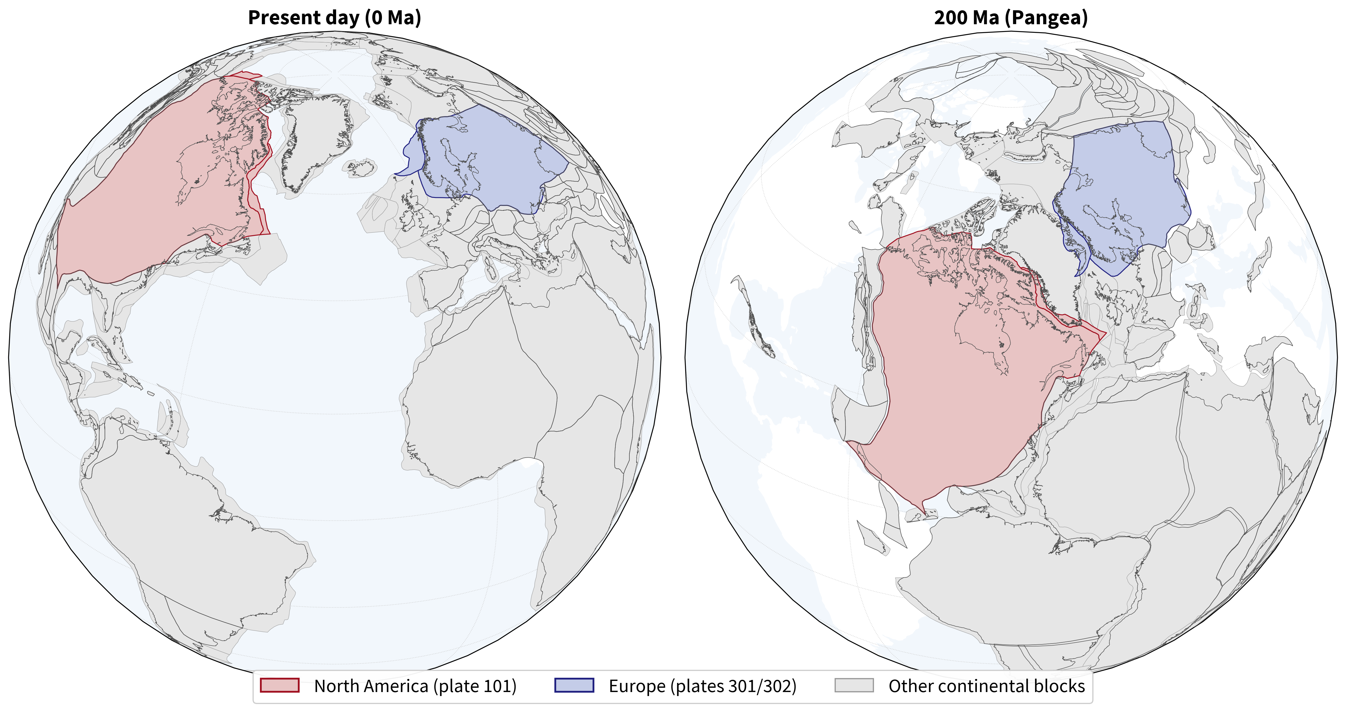
Figure 16.4:Paleogeographic reconstruction using the CEED6 plate model Torsvik & Cocks, 2017 in a paleomagnetic (spin axis) reference frame. a) Present-day configuration. b) 200 Ma (Pangea). North America (red) and Europe (blue) are highlighted; other continental blocks are shown in grey. Coastlines are drawn from the CEED6 land polygon dataset.
Paleomagnetic studies of apparent polar wander provided compelling evidence for continental mobility as early as the 1950s with the idea of drifting continents eventually gaining broad acceptance in the late 1960s, when sea-floor spreading and plate tectonics provided a coherent framework for large-scale lithospheric motion. A classic comparison is between the apparent polar wander paths of North America and Europe when the two continents were joined as part of Pangea prior to the opening of the Atlantic Ocean (Figure 16.4). In their present-day reference frames, the two APWPs diverge significantly (Figure 16.5, left) — the angular distance between coeval poles reaches 15° or more. However, when the European APWP is rotated into the North American reference frame that closes the Atlantic Ocean, the two paths converge (Figure 16.5, right). The angular mismatch drops is much smalled (Figure 16.5, bottom), consistent with the two continents sharing a common polar wander path before the opening of the Atlantic.
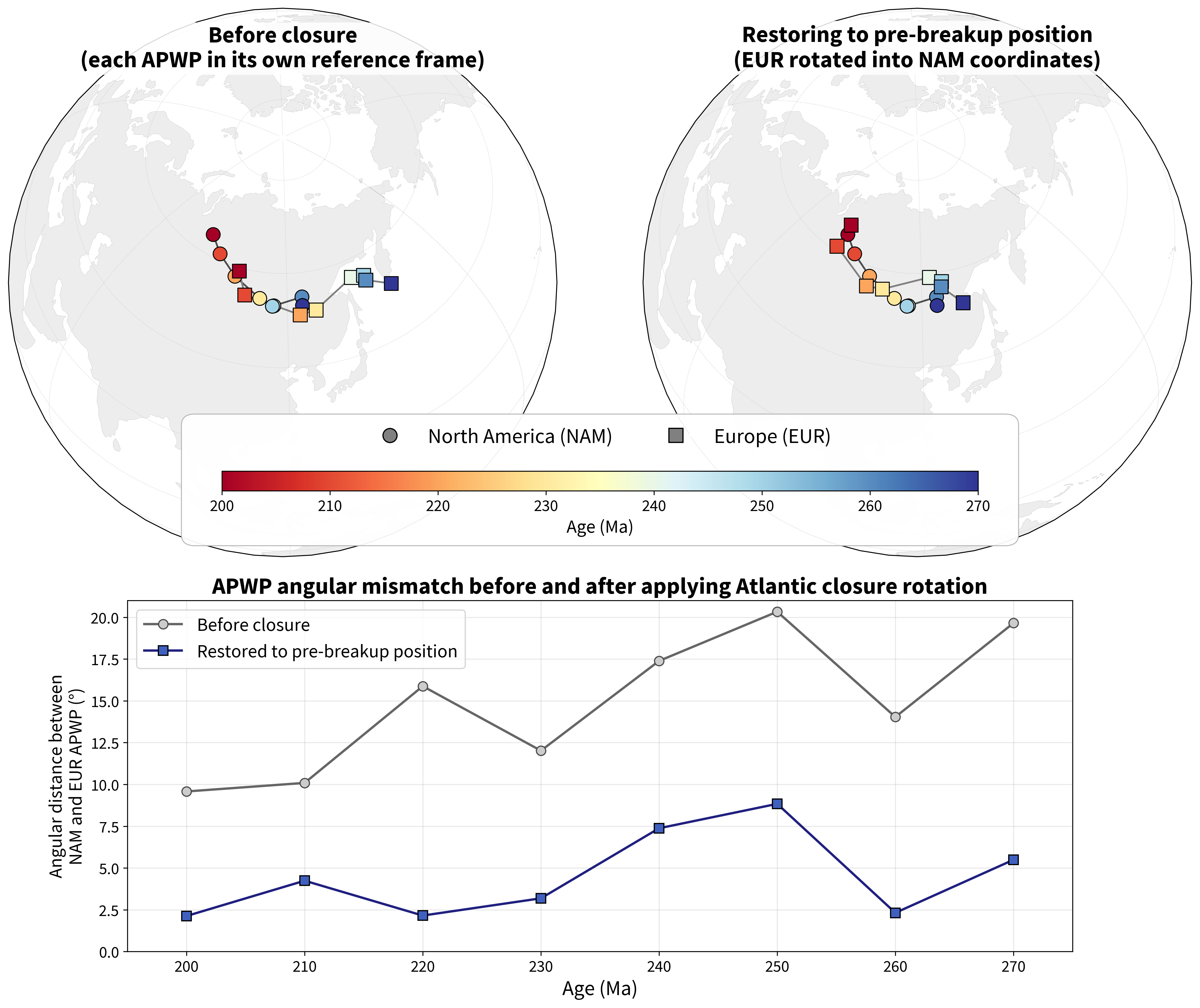
Figure 16.5:Apparent polar wander paths of North America (circles) and Europe (squares) for 200–270 Ma, colored by age. Pole positions are from Torsvik et al. (2012). Left: each APWP in its own present-day reference frame — the paths are separated because the Atlantic Ocean now lies between the two continents. Right: the European APWP rotated into North American coordinates using the age-appropriate finite rotation Torsvik & Cocks, 2017 — the paths converge, consistent with the two continents having been joined within Pangea. Bottom: angular distance between coeval NAM and EUR poles before (grey) and after (blue) applying the closure rotation.
Tremendous effort has been put into compiling finite rotations for various lithospheric plates through time. The most recent and comprehensive compilation is that of Torsvik et al. (2008), which goes back more than 300 Myr. Reconstructions for the last 200 Ma are based mostly on marine geophysical data like marine magnetic anomalies, spreading center and transform azimuths, etc. Pressing back in time, we run out of sea-floor when the Atlantic Ocean is completely closed and finite rotations between blocks must be constrained in other ways, for example, fit of geological observations or paleomagnetic poles. Therefore finite rotations for times prior to about 200 Ma are not independent of the paleomagnetic pole data themselves. Nonetheless, they provide a useful straw man frame of reference. We include a partial list of finite rotations in Section A.3.5.3. Details of how to rotate points on the globe using finite rotations are given in Section A.3.5.3, a technique that will be used extensively in this chapter.
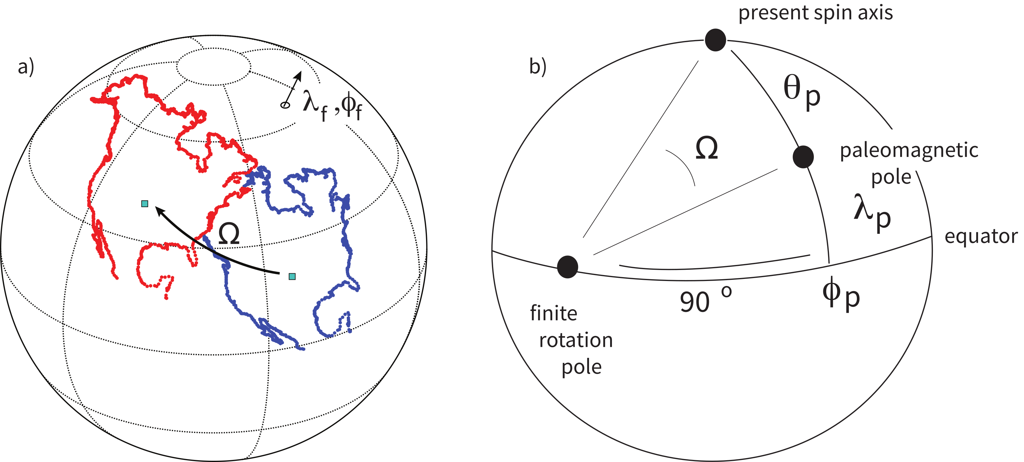
Figure 16.6:a) Finite rotation of North America from one frame of reference to another. Finite rotation pole is located at and the finite rotation is . b) Estimating a finite rotation of a continental fragment from a paleomagnetic pole.
Defining finite rotations based on paleomagnetic poles finds a pole of rotation that transforms the paleomagnetic poles observed on continents back to the spin axis. There are multiple possible finite rotations that achieve this and the problem is inherently non-unique. We show one simple example in Figure 16.6b. The latitude () and longitude () of a finite pole of rotation can be found from a specified paleomagnetic pole () by:
In this way, the points defining a particular continental fragment can be reconstructed to a position consistent with the paleomagnetic pole position; see for example, Figure 16.1a, which is in fact a series of reconstructions of the Indian subcontinent consistent with paleomagnetic poles determined at intervals for the last 80 Ma.
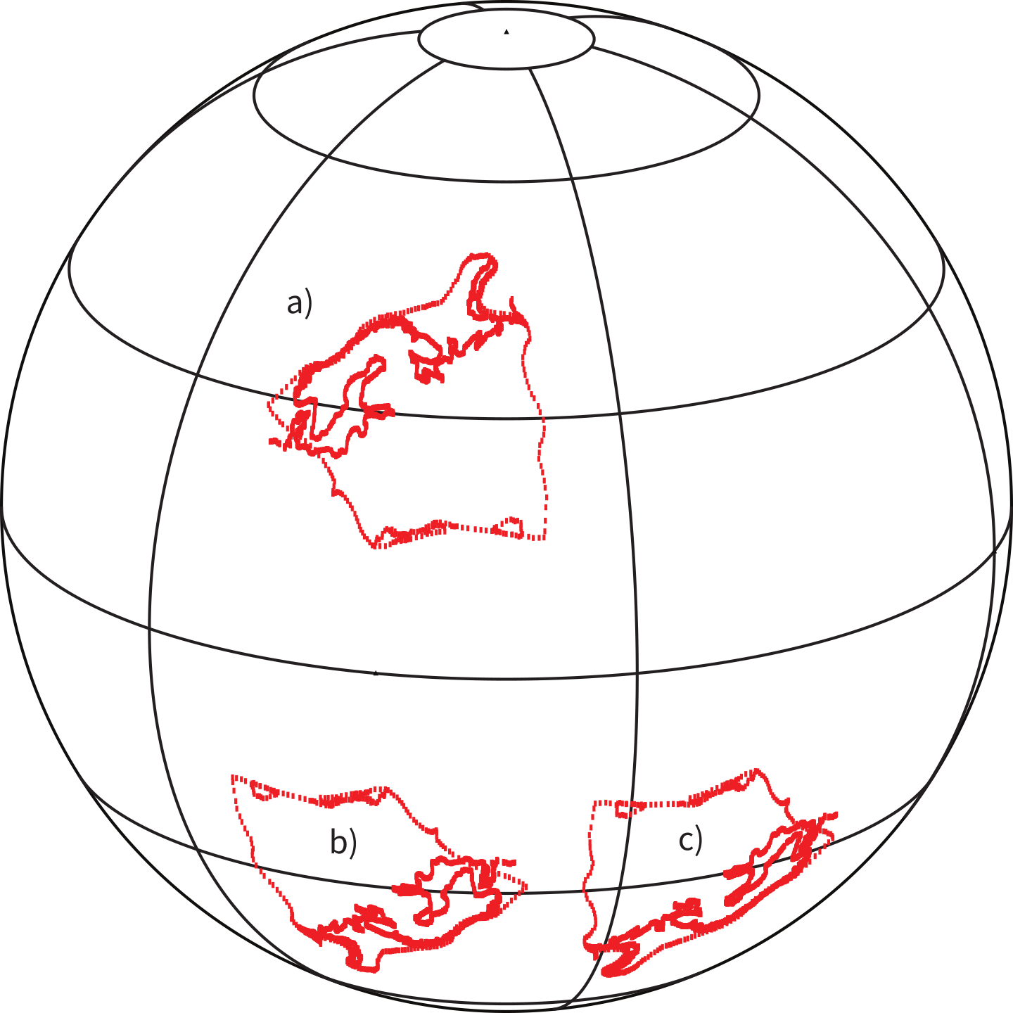
Figure 16.7:Polarity and paleolongitude can be ambiguous from paleomagnetic data alone. All three positions of the continental fragment (a,b,c) could be reconstructions of the same observed direction. a) and b) differ with assumed polarity. b) and c) differ with assumed longitude.
There are two problems with using paleomagnetic poles for constraining finite rotations, however. The first arises from the fact that the paleomagnetic field has two stable states. The two positions labeled a) and b) in Figure 16.7 could have directions that are identical, but the polarity of the observed directions would be opposite. If one had just a snap shot of one of these, without the context tying a particular direction to the North or South pole, it would be impossible to know which was the North seeking direction. In recent times, this is not a problem because such a context exists, but in the Precambrian and early Paleozoic, the context can be lost and the polarity can be ambiguous. The second problem with using paleomagnetic poles for constraining finite rotations is that paleo-longitude cannot be constrained from the pole alone; the two positions labelled b) and c) in Figure 16.7 are equally well fit by a given paleomagnetic pole.
16.2Poles and Apparent Polar Wander
16.2.1Calculating a Paleomagnetic Pole
In Chapter 2, we introduced the virtual geomagnetic pole (VGP) — the position of the equivalent magnetic pole calculated from a single observation of the field direction at a known location using the dipole formula. A collection of VGPs from multiple lava flows or other independent records of the geomagnetic field, obtained from rocks of similar age, can be averaged to yield a paleomagnetic pole. If the data set includes enough independent recordings of the field, paleosecular variation is effectively averaged out and the resulting mean pole approximates the position of the geographic (spin) axis as viewed from the sampling locality. When both normal and reversed polarity directions are present, one polarity must be flipped to the other (by taking the antipode) before averaging, so that all VGPs cluster in the same hemisphere.
Once a paleomagnetic pole has been determined, it provides a direct constraint on the paleolatitude of the sampling locality. The angular distance from the study location to the paleomagnetic pole is the paleomagnetic colatitude. The paleolatitude of the site is simply 90° minus the colatitude — equivalent to the angular distance from the site to the paleoequator, the great circle 90° from the pole (see Figure 16.8). Because the time-averaged geomagnetic field is axially symmetric under the GAD assumption, paleomagnetic data constrain paleolatitude but not paleolongitude — a fundamental limitation that we will return to throughout this chapter. Similarly, the polarity ambiguity means that a pole position and its antipode are equally valid without independent constraints on which hemisphere the continent occupied.
As a concrete example, Figure 16.8 shows a paleomagnetic pole calculated from 59 reversed polarity lava flows of the upper Osler Volcanic Group (ca. 1105 Ma), erupted during the Midcontinent Rift and exposed along the north shore of Lake Superior Halls, 1974Swanson-Hysell et al., 2014. The individual VGPs scatter about the mean pole — a consequence of paleosecular variation recorded by successive flows. The colatitude from the study location to the pole is 47.9°, yielding a paleolatitude of 42.1°N and indicating that this part of Laurentia was at mid-latitudes at ca. 1105 Ma.
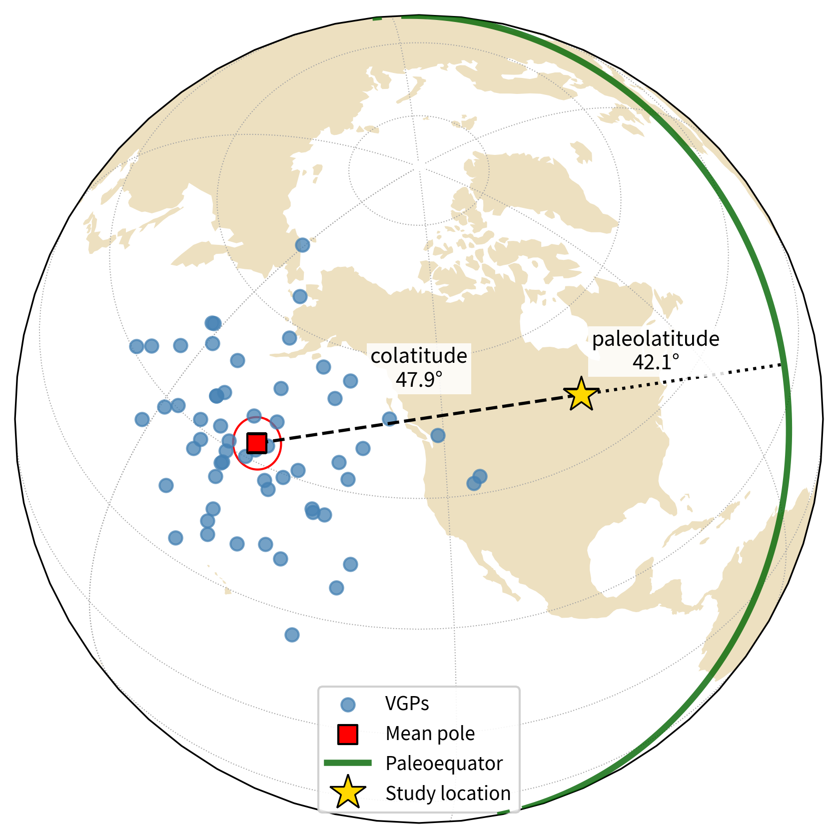
Figure 16.8:Virtual geomagnetic poles (VGPs; blue circles) calculated from tilt-corrected site-mean directions of 59 reversed polarity lava flows of the upper Osler Volcanic Group (ca. 1105 Ma), flipped to normal polarity. The red square marks the Fisher mean paleomagnetic pole (42.5°N, 201.6°E, A = 3.7°, N = 59) with its 95% confidence circle. The gold star is the study location on the north shore of Lake Superior. The green great circle is the paleoequator — the locus of points 90° from the paleomagnetic pole. The dashed line from the pole to the study location spans the paleomagnetic colatitude (47.9°), while the dotted line from the study location to the paleoequator spans the paleolatitude (42.1°).
The goal of much paleomagnetic research has been to assemble the various poles or some subset of poles into apparent polar wander paths (APWPs) for the many different continental fragments. There are two issues that guide the construction of APWP: selection of poles which can be considered “reliable” and curve fitting.
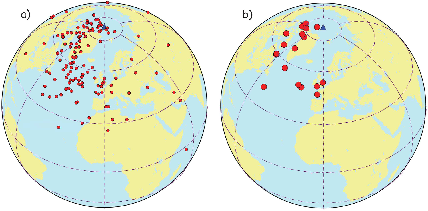
Figure 16.9:Paleomagnetic poles from Australia for the last 200 Ma from GPMDB. a) No selection criteria. b) The selection criteria of BC02.
Picking out the meaningful poles from the published data is part of the art of paleomagnetism. We have been building a tool kit for dealing with this problem throughout this book. There is some agreement in what constitutes a “good” pole among various workers. The general selection criteria used by most paleomagnetists are based on those summarized by Voo (1990). They have been modified for particular applications, for example, by Besse & Courtillot (2002).
The age of the formation must be known rather accurately. In the V90 criteria, the age should be known to within a half of a geological period (see Chapter 15) or within a numerical age of ± 4% for Phanerozoic data. For Precambrian rocks, the age should be known to within ± 4% or 40 Myr, whichever is smaller. Some applications require that poles be rotated from one continental reference frame to another, which demands tighter age constraints. For example, Besse & Courtillot (2002) set age uncertainties of 15 Myr.
In order to average errors in orientation of the samples and scatter caused by secular variation, there must be a sufficient number of individually oriented samples from enough sites. What constitutes “sufficient” and “enough” here is somewhat subjective and a matter of debate. The V90 Criteria recommend a minimum of 24 discrete samples of the geomagnetic field each having a . Some authors also compare scatter within and between sites in order to assess whether secular variation has been sufficiently sampled, but this relies on many assumptions as to what the magnitude of secular variation was (see Chapter 14). Butler (1992) suggested using the scatter of VGPs ( in Chapter 14) to decide whether secular variation has been averaged out or whether there is excess scatter in the data set. Besse & Courtillot (2002) recommend using only poles with at least six sites and 36 samples, each site having a 95% confidence interval less than 10° in the Cenozoic and 15° in the Mesozoic.
It must be demonstrated that a coherent characteristic remanence component has been isolated by the demagnetization procedure. McElhinny & McFadden (2000) attempted to standardize the description of the demagnetization status of a dataset using a demagnetization code (DC) (see Table 16.1). Besse & Courtillot (2002) recommend using only poles with a DC of at least 2.
The age of the magnetization relative to the age of the rock should be constrained using field tests (fold test, conglomerate test, baked contact test, see Chapter 9). Besse & Courtillot (2002) reject poles that fail a fold test or a reversals test.
There should be agreement in the pole positions from units of similar age from a broad region and adequate knowledge of any structural corrections necessary. Besse & Courtillot (2002) reject poles from “mobile regions”, but incorporate data that are azimuthally unconstrained by using inclination only data as a constraint on paleolatitude (see Section 16.7 for a more complete discussion).
Both polarities should be represented and the two data sets should be antipodal.
Pole positions should not fall on a younger part of the pole path or on the present field direction. Such poles should be viewed with suspicion.
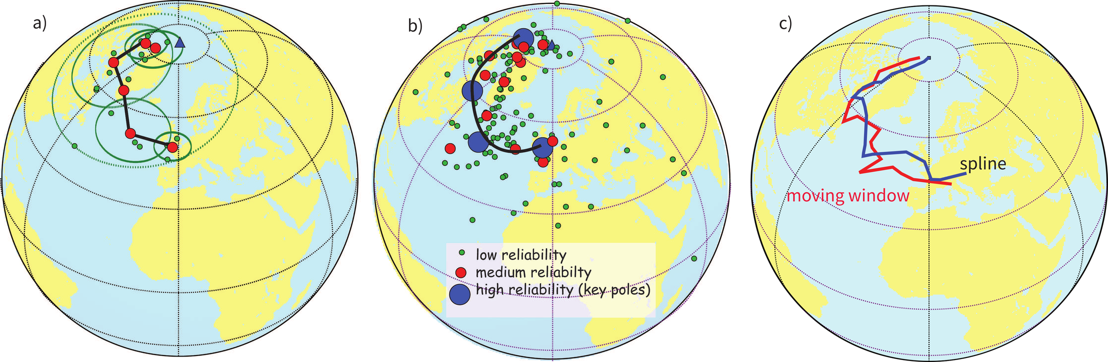
Figure 16.10:Examples of how to construct an APWP. a) Discrete window. b) Key pole approach. c) Moving window Besse & Courtillot, 2002 versus spline Torsvik et al., 2008.
Table 16.1:Demagnetization Codes (DC) summarized by McElhinny & McFadden (2000).
| DC | Description |
|---|---|
| 0 | Only NRM values reported. No evidence for demagnetization. |
| 1 | Only NRM values reported. Demagnetization on pilot specimens suggest stability. |
| 2 | Demagnetization at a single step on all specimens. No demagnetograms shown. |
| 3 | Demagnetograms shown that justify demagnetization procedure chosen. |
| 4 | Principal component analysis (PCA) carried out from analysis of Zijderveld diagrams. (see Chapter 9) |
| 5 | Magnetic vectors isolated using two or more demagnetization methods with PCA, e.g., thermal and AF demagnetization (see Chapter 9). |
In the V90 criteria, each pole gets a point for every criterion that it passes. The sum of the points is the quality factor which ranges from 0 to 7. It is not expected that every pole satisfy all seven criteria (very few would!). Most authors use poles with . Besse & Courtillot (2002) on the other hand use criteria 1-5 (must have all of them) but do not require 6 or 7.
In order to understand the process of constructing APWPs, we will begin with the plot of all the paleomagnetic poles from Australia for the last 200 Myr (Figure 16.9). These poles form a smear that extends in a broad arc away from the spin axis down the Atlantic and then into Europe and Africa. Of the 137 poles from Australia in the GPMDB plotted in Figure 16.9a, only 18 meet the BC02 criteria (see Figure 16.9b). These form a sparse track which could form the basis for an APWP.
Once selected, the poles must be combined together somehow in order to define an apparent polar wander path for any of the continental fragments. The goal of this process is to produce a list of paleomagnetic poles at more or less uniform time intervals for each independent lithospheric fragment. There have been several different approaches to this problem in the literature as summarized below:
Discrete windows (Figure 16.10a): Selected poles for a given continent or continental fragment are separated into discrete time intervals and poles in each time window are averaged. There is no overlap of poles between windows so each window is independent of the others.
Key poles: Practitioners identify what are considered to be the most reliable poles, so-called “key poles” (e.g., largest dots in Figure 16.10b). If the data quality is highly uneven, key poles can be used as anchor-points.
Moving windows: Same as (1), but time windows overlap and paleopoles can be included in more than one window. Successive mean poles are not independent of each other (see Figure 16.10c).
Fitting curves with splines: This technique fits a smoothly curving path to the available paleopoles Jupp & Kent, 1987, some of which can be weighted more than others (see Figure 16.10c).
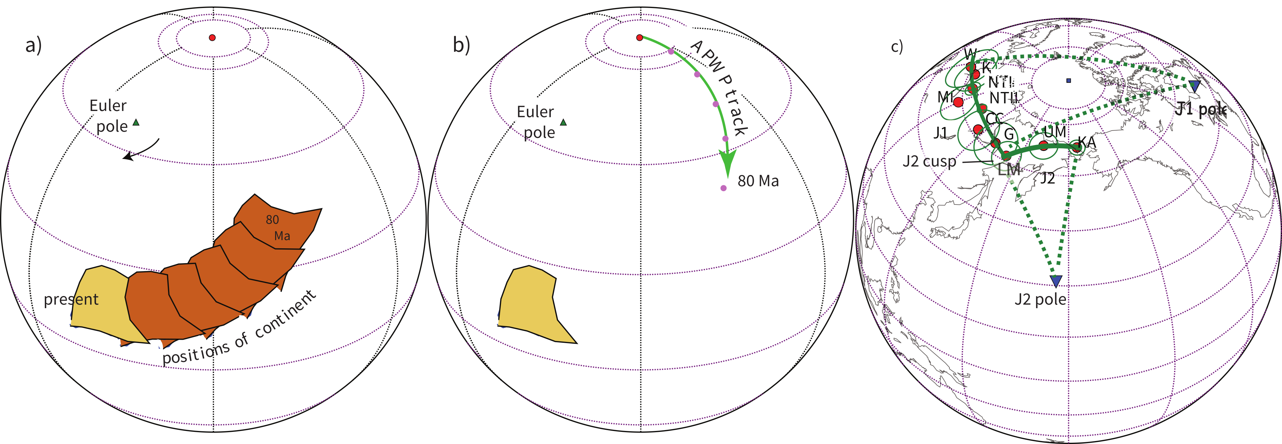
Figure 16.11:a) Paleomagnetic Euler pole method for determining APWPs. A continent is rotating about a fixed Euler pole (green triangle). As the continent moves, rocks record paleomagnetic directions reflecting the position of the spin axis at that particular age. b) When viewed in the present coordinate system and converted to paleomagnetic poles, these will fall on the small circle APWP track. c) PEP analysis for Jurassic APWP for North America of May & Butler (1986). Poles are interpreted to lie along small circle tracks (J1/J2) separated by a cusp (J2 cusp) located at the LM pole. The J1 and J2 tracks are small circles about their respective Euler poles, shown as blue triangles.
PEP analysis: Paleomagnetic Euler Pole analysis assumes that APWP segments are small circles about an Euler pole Gordon et al., 1984; see Figure 16.11a. The underlying assumption is that the continents move according to the same Euler vector for considerable stretches of time (e.g., 10 years). When viewed from the continental frame of reference, the poles plot along an apparent polar wander path that forms a small circle about the Euler pole (Figure 16.11b). May & Butler (1986) applied the technique to the North American APWP. Their compilation of Jurassic key poles is shown in Figure 16.11c. These were interpreted to lie along two tracks (J1 and J2) separated by a cusp (J2 cusp) at the LM (Lower Morrison Formation) pole. Each track is a small circle about its respective Euler pole (shown as blue triangles). We will return to this topic in Section 16.7.
Master path: The “master path” approach (e.g., Besse & Courtillot (2002); Torsvik et al. (2008)) argues that if the rotation parameters between continents are well known as a function of age, then poles from one continent can be transferred to the coordinate system of another. When all suitable poles are transferred to a single continent they can be used to constrain a single synthetic apparent polar wander path by, for example, windowing or spline fitting. The synthetic path can then be exported back to the contributing continents (see, e.g., Figure 16.12e).
Use of inclination only data from regions suspected of local rotations. Even if a region has undergone local rotation, the inclinations provide constraints for paleolatitude. The paleomagnetic pole must lie on the paleolatitude small circle around the site location. These small circles can be used to supplement fully oriented paleopoles, or if there are enough data from sufficiently disparate locations, a unique intersection can be used to define the position of the paleomagnetic pole (see Figure 16.13).
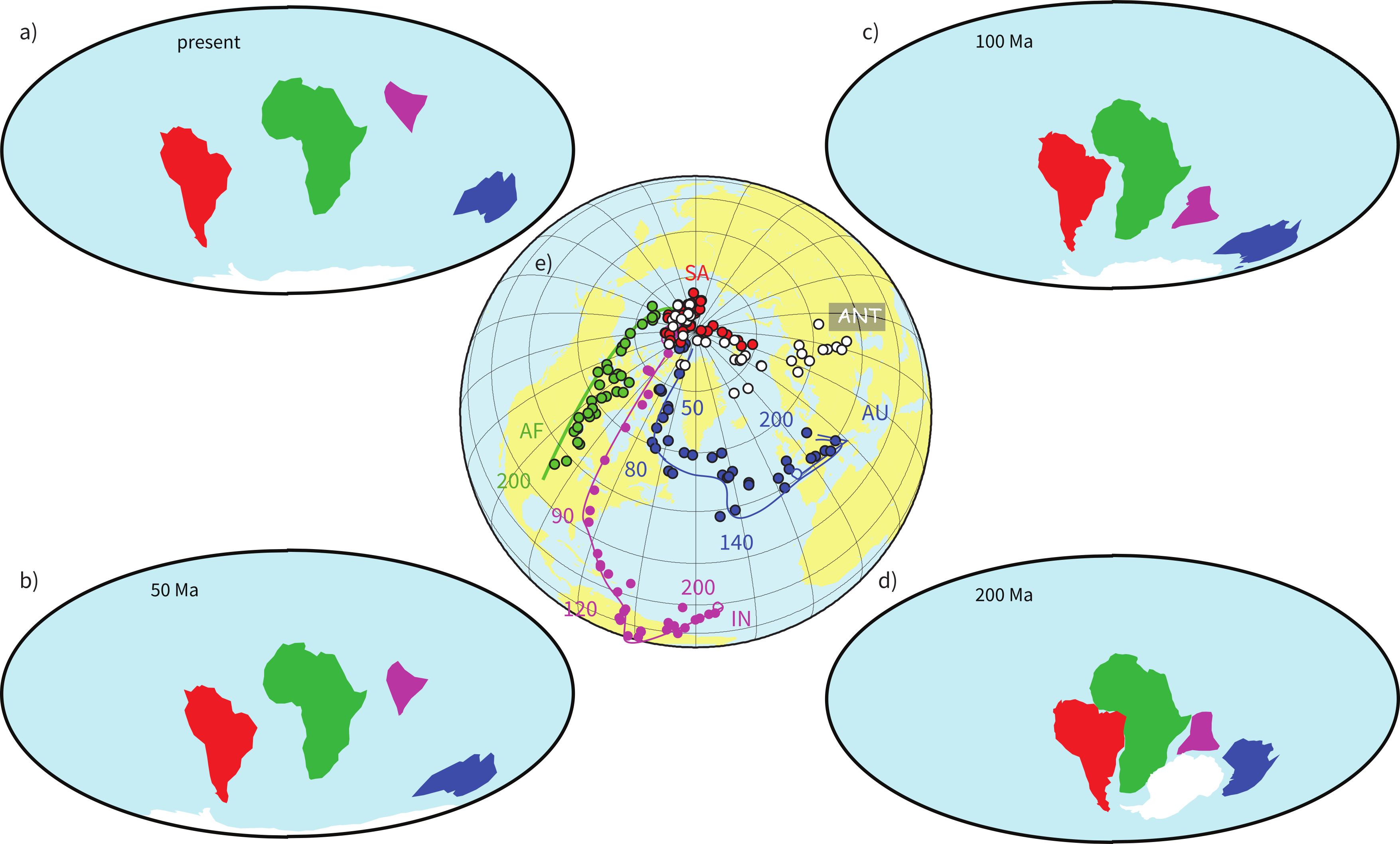
Figure 16.12:Master path approach: Maps of continental reconstructions for a) present, b) 50, c) 100, and d) 200 Ma. e) Poles and APWP for various continents for the last 200 million years, evaluated at five million year intervals. [Reconstructions using finite rotation poles of Torsvik et al. (2008) (see Section A.3.5.3).] Paleomagnetic poles from the synthetic APWP constructed by Besse & Courtillot (2002) exported to the different continents.
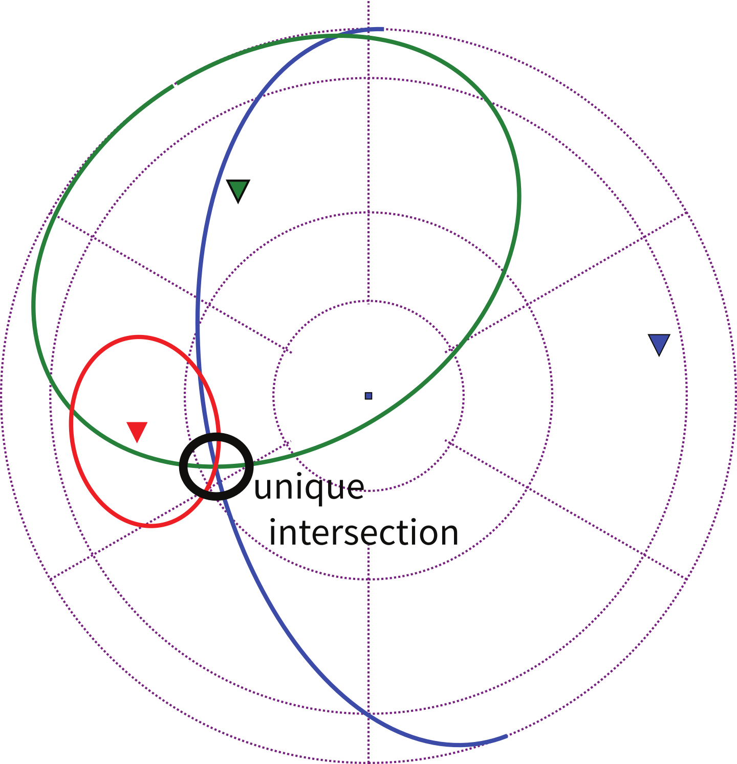
Figure 16.13:Sampling sites are marked by triangles. Inclinations from the sites can be used to calculate the paleomagnetic colatitude of the site using the dipole formula (see Chapter 2) which defines a small circle along which the paleomagnetic pole must lie. The intersection of three such small circles uniquely defines the position of the paleomagnetic pole.
16.3The Gondwana APWP
Besse & Courtillot (2002) produced a master path for the last 200 Myr and Torsvik et al. (2008) refined the poles of rotation and extended them back to 320 Ma. Prior to about 200 Ma, however, rotation poles are more difficult to constrain, independent of the paleomagnetic data themselves. Both the quality and quantity of the available poles decline with increasing age. The assumptions of the GAD hypothesis and amount and style of secular variation become increasingly problematic. Furthermore, most continents are composed of separate blocks whose relationships in ancient times are unknown or poorly known. Exceptions to this are supercontinents like Gondwana for which it is possible to combine data from different blocks with some confidence.
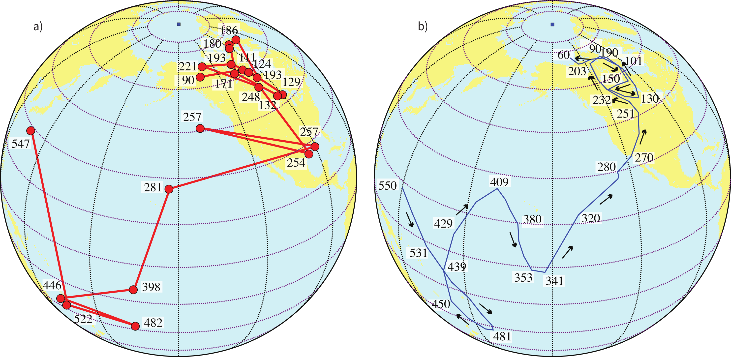
Figure 16.14:The South African APWP for the Phanerozoic. a) South African poles only (Table 1 of Torsvik & Voo (2002)). b) Smoothed APWP spline path using master path approach for Gondwana in South African coordinates.
Gondwana was a supercontinent that coalesced about 550 Ma and was incorporated into a larger supercontinent of Pangea during the Carboniferous. Pangea itself began breaking up during the Mid-Jurassic when the Atlantic Ocean began to form. The core continental fragments that comprise Gondwana are NE, NW and Southern Africa, South America, Madagascar, Greater India, Cratonic Australia and East Antarctica. Torsvik & Voo (2002) compiled a list of paleomagnetic poles from these core parts of the Gondwana continents ( for the V90 criteria) along with a set of finite rotation poles for putting them back together.
As an example of the kind of pole paths available for an individual continent, we show all the poles selected by Torsvik & Voo (2002) from the South African continental fragment in Figure 16.14a. The inferred path is quite complicated in the Mesozoic and the poles are sparse prior to about 250 Ma leading to the suspicion that the path is somewhat undersampled. By rotating poles from all the Gondwana continental fragments into South African coordinates and fitting them with a smoothed path using splines, Torsvik & Voo (2002) produced the APWP shown in Figure 16.14b.
Pushing back to times before Gondwana gets increasingly difficult because indigenous poles become more sparse and more poorly dated and reconstruction of the pre-Gondwana continental bits becomes less well constrained. Nonetheless, some authors have pushed their interpretations of Cambrian data to rather extreme conclusions. For example, large swings in the APWP for Australia led to the conclusion that the entire spin axis of the Earth changed by 90° suddenly in a feat termed “inertial interchange true polar wander” (see, e.g., Kirschvink et al. (1997)).
16.4Inclination Shallowing and GAD
One of the most useful, in fact essential, assumptions in paleomagnetism is that the geomagnetic field is on average closely approximated by a geocentric axial dipole (GAD). As discussed in Chapter 14, the GAD hypothesis has been found to be nearly true for at least the last 5 million years with the largest non-GAD contribution to the spherical harmonic expansion generally being of the order of 5%. For the more ancient past, it is difficult to test the GAD (or any other field) hypothesis owing to plate motions, accumulating problems of overprinting, and difficulty in reconstructing paleo-horizontal. Although most paleomagnetic studies make the implicit assumption of a GAD field, several recent studies have called the essential GAD nature of the ancient field into question. These studies fall into two groups: those that use reference poles and plate tectonic reconstructions to predict directions (e.g., Si & Voo (2001)) and those that compare observed statistical distributions of directions to those predicted by different field models (e.g., Kent & Smethurst (1998); Voo & Torsvik (2001)). The inescapable conclusion from these and other studies is that there is often a strong bias toward shallow inclinations and many studies have called on non-dipole field contributions, in particular large (up to 20%) average zonal octupole () contributions (see Chapter 2 and Chapter 14). We will explore these ideas in the following.
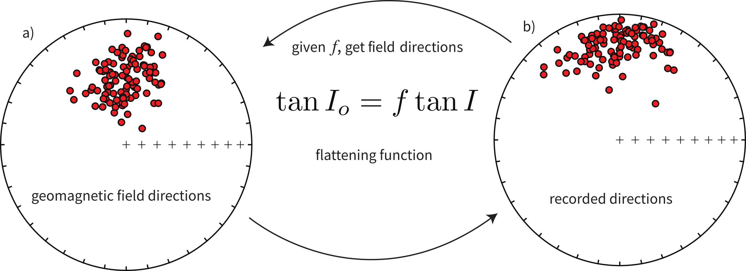
Figure 16.15:a) Set of possible geomagnetic field directions plotted in equal area projection. Lower (upper) hemisphere directions are solid (open) symbols. b) Directions recorded by the sediment using the flattening function. [Figure modified from Tauxe et al. (2008).]
From Chapter 14 we know that paleomagnetic directions from the last five million years are, if anything, elongate in the North-South vertical plane. However, sedimentary inclination flattening not only results in directions that are too shallow, but also reduces N-S elongations in favor of elongations that are more east-west. This effect is shown in Figure 16.15. Geomagnetic field directions (e.g., Figure 16.15a) with inclinations are recorded in sediments with observed inclinations () following the flattening function of King (1955) (see Chapter 7), , where is the flattening factor ranging from unity (no flattening) to 0 (completely flattened). Examples of the recorded “flattened” directions are shown in Figure 16.15b. Note that flattened directions tend to become elongate in the horizontal plane, a feature that distinguishes this cause of inclination shallowing from others, for example, poleward plate motion which leaves the distribution unchanged or non-dipole field effects. Zonal non-dipole field contributions like those from axial quadrupole or octupole fields make the distribution more elongate in the meridional plane (see, e.g., Tauxe & Staudigel (2004)).
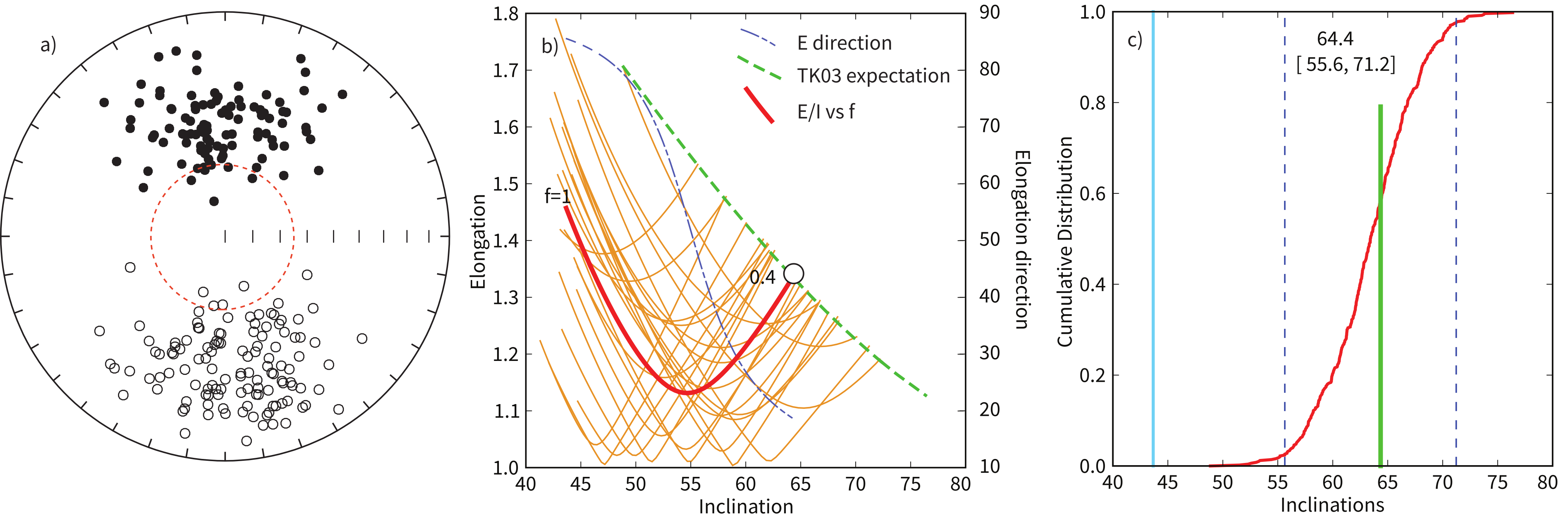
Figure 16.16:a) Paleomagnetic directions of Oligo-Miocene redbeds from Asia in equal area projection (stratigraphic coordinates). [Redrawn from Tauxe & Staudigel (2004); data from Gilder et al. (2001).] b) Plot of elongation versus inclination for the data (heavy red line) and for the TK03.GAD model (dashed green line). Also shown are results from 20 bootstrapped datasets (yellow). The crossing points represents the inclination/elongation pair most consistent with the TK03.GAD model. Elongation direction is shown as a dash-dotted (purple) line and ranges from E-W at low inclination to more N-S at steeper inclinations. c) Cumulative distribution of crossing points from 5000 bootstrapped datasets. The inclination of the whole data set (64.4°) is consistent with that predicted from the Besse & Courtillot (2002) European APWP. The 95% confidence bounds on this estimate are 55.6-71.2°.
Earlier in the chapter, we discussed the BC02 APWPs for the major continents. These can be used to predict directions for a given time and place using the spherical trigonometric tricks covered in Section A.3.1. Despite the general success of the BC02 APWPs for predicting directions, comparison of predicted directions with those observed in many data sets from red beds in Central Asia led some authors to the conclusion that the GAD hypothesis had failed. We show an example of such a data set in Figure 16.16a, although it is atypical in that there are an unusually large number of directions. These have a mean of = 356.1°, = 43.7°. Assuming that the location of the study (presently at 39.5°N, 94.7°E) has been fixed to the European coordinate system and taking the 20 Myr pole for Europe from Besse & Courtillot (2002) (81.4°N, 149.7°E), the inclination is predicted to be 63° (see dashed curve in Figure 16.16a). These sediments are typical of Asian sedimentary units in having an inclination relative to the predicted values that is some 20° too shallow.
The elongation-inclination (E/I) method of detecting and correcting inclination shallowing of Tauxe & Staudigel (2004) (see also Tauxe et al. (2008)) simply “unflattens” observed directional data sets using the inverse of the flattening formula and values for ranging from 1 (no unflattening) to 0.4. At each unflattening step, we calculate inclination and elongation ( of the orientation matrix, see Section A.3.5.4) and plot these as in Figure 16.16a. We know from Chapter 14 that elongation decreases from the equator to the pole, while inclination increases; A best-fit polynomial through the inclination - elongation data from model TK03.GAD is: (as recalculated by Tauxe et al. (2008)) and is shown as the green line in Figure 16.16b. There is a unique pair of elongation and inclination that is consistent with the TK03.GAD field model (circled in Figure 16.16b) with an inclination of 64°. As goes from 1 to 0.4, the inclination of the unflattened directions increases from about 45° to about 65°. At the same time the direction of elongation (dash-dotted line -- see right hand vertical axis label) changes systematically from East-West (85°) to more North-South (15°).
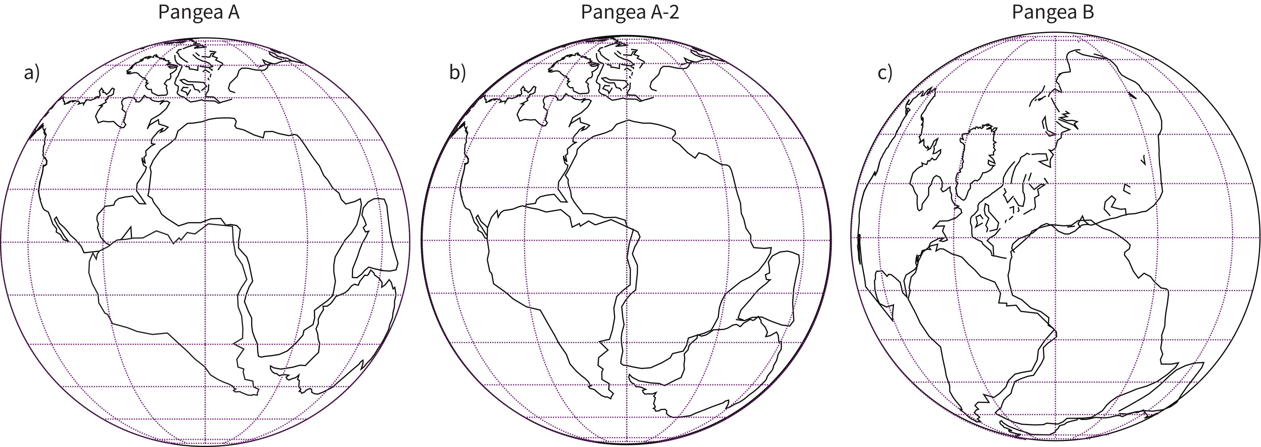
Figure 16.17:a) Pangea A reconstruction (“Bullard fit”; Smith & Hallam (1970); Bullard et al. (1965)). b) Pangea A-2 reconstruction Voo & French, 1974. c) Pangea B reconstruction Morel & Irving, 1981. Note: a) and b) are reconstructions to fit the continental margins and do not take into account paleolatitudes.
To obtain confidence bounds on the “corrected” inclination, the E/I method performs a bootstrap (see Section A.3.7). E/I curves from twenty such bootstrapped data sets are shown as thin lines in Figure 16.16b. A cumulative distribution curve of 5000 crossing points of bootstrap curves with the model elongation-inclination line are plotted in Figure 16.16c. The average inclination of the original (uncorrected) data is shown as the light blue line in the plot and the corrected inclination as the heavy green line at 64.4°. The 95% confidence bounds are shown as dashed lines at 55.6 and 71.2°. The E/I corrected inclination is consistent with that predicted by the BC02 path for stable Europe.
Tan et al. (2003) performed the AARM correction (see Chapter 13) on the Tarim red beds and found a similar correction factor. Hence AARM correction (which is labor intensive in the lab) and EI correction (which is labor intensive in the field) give similar results. Both methods strongly suggest that inclination shallowing in the Asian red beds is indeed caused by sedimentary inclination shallowing of the type described in Chapter 7.
Table 16.2:Rotation poles for various versions of Pangea.
| AF | AUS | ANT | IND | SAM | ||||||
|---|---|---|---|---|---|---|---|---|---|---|
| # | ||||||||||
| 1 | -4 | 40 | -31 | 1 | -36 | 58 | 29 | |||
| 2 | 0 | 0 | 0 | 1 | -36 | 58 |
| # | |||||||||||||||
|---|---|---|---|---|---|---|---|---|---|---|---|---|---|---|---|
| 1 | -4 | 40 | -31 | 1 | -36 | 58 | 29 | 42 | -59 | 44 | -31 | 57 | |||
| 2 | 1 | -36 | 58 | ||||||||||||
| 3 | 19 | -1 | -20 | 19 | -1 | -20 | 19 | -1 | -20 | 19 | -1 | -20 | 19 | -1 | -20 |
| # | |||||||||||||||
|---|---|---|---|---|---|---|---|---|---|---|---|---|---|---|---|
| 1 | -4 | 40 | -31 | 1 | -36 | 58 | 29 | 42 | -59 | 44 | -31 | 57 | |||
| 2 | 1 | -36 | 58 | ||||||||||||
| 3 | 0 | 147 | 50 | 0 | 147 | 50 | 0 | 147 | 50 | 0 | 147 | 50 | 0 | 147 | 50 |
| NAM | EUR | GRN | ||||
|---|---|---|---|---|---|---|
| # | ||||||
| 1 | 68 | -14 | 75 | |||
| 2 | ||||||
| 3 |
| # | |||||||||
|---|---|---|---|---|---|---|---|---|---|
| 1 | 68 | -14 | 75 | 89 | 28 | -38 | |||
| 2 | 68 | -14 | 75 | ||||||
| 3 | |||||||||
| 4 | 0 | 129 | 47 | 0 | 138 | 58 | |||
| 5 | -90 | 0 | 31 | -90 | 0 | 36 |
Gondwana Continents:
Pangea A: Bullard et al. (1965), Smith & Hallam (1970)
Pangea A-2: Voo & French (1974)
Pangea B: Morel & Irving (1981)
Laurasian Continents:
Pangea A: Bullard et al. (1965), Smith & Hallam (1970)
Pangea B: Morel & Irving (1981)
#: Rotation number. Rotations performed in order using algorithm in Section A.3.5.3. are the latitude, longitude and angle of the finite rotation pole. AF: Africa, AUS: Australia, ANT: East Antarctica, IND: India, SAM: South America, NAM: North America, EUR: Europe and GRN: Greenland.
16.5Paleomagnetism and Plate Reconstructions
In addition to defining finite rotations for reconstruction, paleomagnetic poles can be used as an independent test of proposed reconstructions based on other observations. After reconstructing continental fragments according to some hypothesized set of finite rotations, one can assess whether the paleomagnetic poles are consistent with such a reconstruction. Are the poles better clustered in one reconstruction as opposed to another? Do poles from separate continental blocks fall on top of each other after reconstruction? If the paleomagnetic poles are not well clustered, then there must be something wrong with the poles themselves, the reconstruction, or the GAD hypothesis; arguments about particular reconstructions revolve around all three of these issues. As an example of the role of paleomagnetic poles in paleogeographic reconstructions, we consider the case of Pangea, a topic of debate for over three decades.
Many people who have contemplated the globe have had the desire to fit North and South America against Europe and Africa by closing the Atlantic Ocean. One such attempt, known as the Bullard fit Bullard et al., 1965, fits the continents together using minimization of misfits (gaps and overlaps) of a particular contour on the continental shelves as the primary criterion. This reconstruction (extended by Smith & Hallam (1970)) has come to be called the Pangea A (also known as A-1) fit and is shown in Figure 16.17a. There is little controversy over this fit as the starting point for the opening of the Atlantic in the Jurassic. The fit is strongly supported by paleomagnetic data as shown in Figure 16.18a in which we plot poles from the time period spanning 180 to 200 Ma from the lists of Besse & Courtillot (2002) and Torsvik et al. (2008). These poles have been rotated into the Pangea A reference frame using the poles of rotation listed in Table 16.2 for each continent.
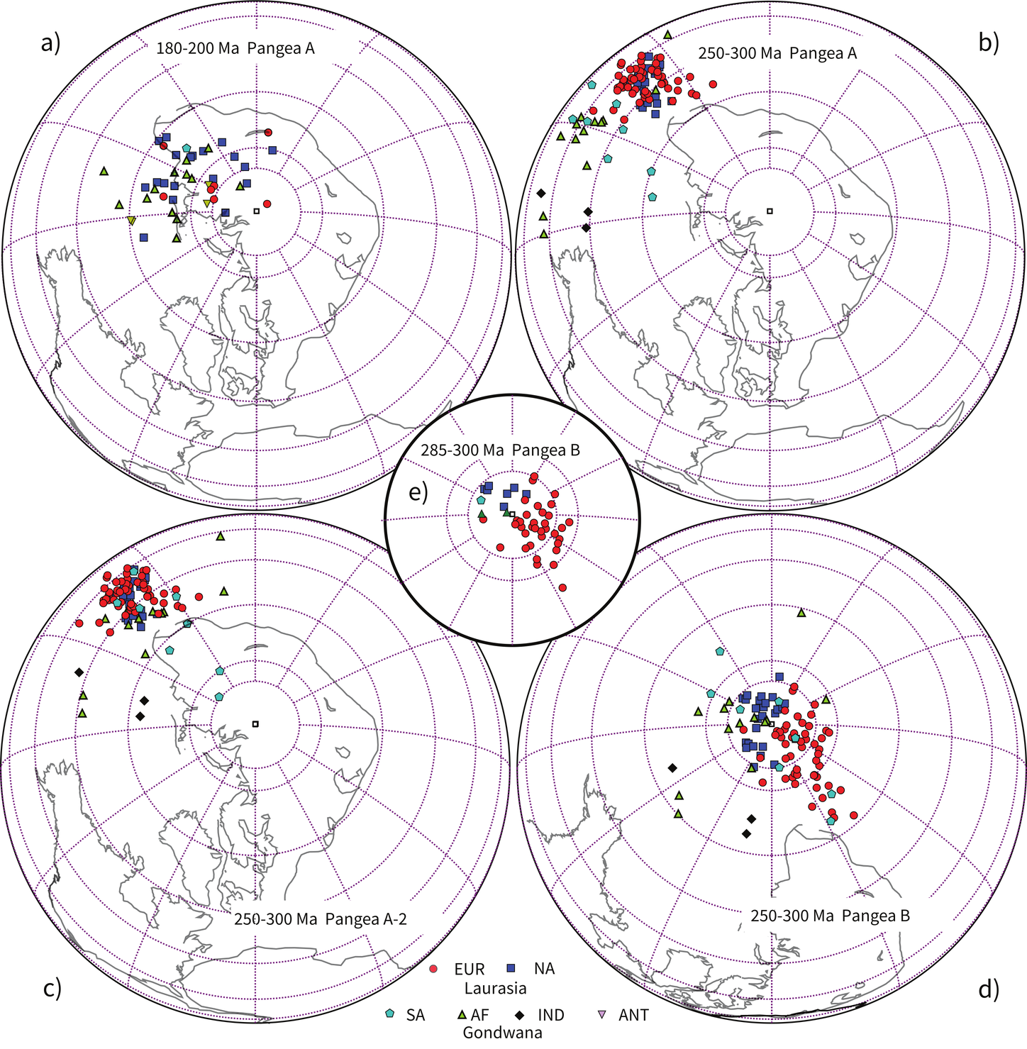
Figure 16.18:Using paleomagnetic poles as a test for reconstructions. The continental outlines are rotated according to the same finite rotation poles for each reconstruction (in light grey). a) Poles for the period 180-200 Ma Pangea from the Besse & Courtillot (2002) and Torsvik et al. (2008) compilations rotated to the Pangea A reconstruction of Bullard et al. (1965) and Smith & Hallam (1970). b) Poles for the Permian (250-300 Ma) from Torsvik et al. (2008) compilation shown in Pangea A reconstruction. c) Same as b) but for Pangea A-2 reconstruction of Voo & French (1974). d) same as b) but for Pangea B reconstruction Morel & Irving, 1981. e) Same as d) but just the lower Permian poles.
The ink was scarcely dry on the Smith & Hallam (1970) version of Pangea A when paleomagnetists began exploring its limits. Voo & French (1974) pointed out that data from the older parts of Gondwana (Paleozoic to perhaps Early Triassic) did not fit as well as the younger parts. We show poles from the Permian (250-300 Ma) compiled by Torsvik et al. (2008) in Figure 16.18b after rotation to the Pangea A frame of reference. The poles are more scattered and there is a systematic separation of poles from Gondwana continents relative to those from Laurasia. Voo & French (1974) modified the Pangea A fit (Pangea A-2) which improved the clustering of the poles (see Figure 16.17b and Figure 16.18c). An entirely different solution was proposed by Irving (1977) and Morel & Irving (1981), known as Pangea B (see Figure 16.17). This fit takes advantage of the non-uniqueness of longitude in paleomagnetic reconstructions and slides North America to the west of South America. The resulting pole distribution is shown in Figure 16.18d. Pangea B must then transform to Pangea A at some point before the opening of the Atlantic. Muttoni et al. (2003) advocated a reconstruction much like Pangea B and suggested that it began to evolve toward Pangea A-2 by the mid Permian. In Figure 16.18e, we show poles from just the lower Permian (285-300 Ma). While the (lower) Permian poles from most continents do agree with the Pangea B fit, those from Europe (red dots) are significantly offset. Interestingly, the North American poles do not agree with the European poles either, so there must be some problem in the reconstruction of Laurasia in the Pangea B reconstruction.
16.6Discordant Poles and Displaced Terranes
Regions with paleomagnetic directions that are different from that expected from the reference pole of the APWP may have rotated or translated from their original positions as independent entities (as tectonostratigraphic terranes or microplates). As workers began investigations in the western parts of North America, it soon became apparent that many of the poles were well off the beaten track for the rest of the plate (see, e.g., Irving (1979)).
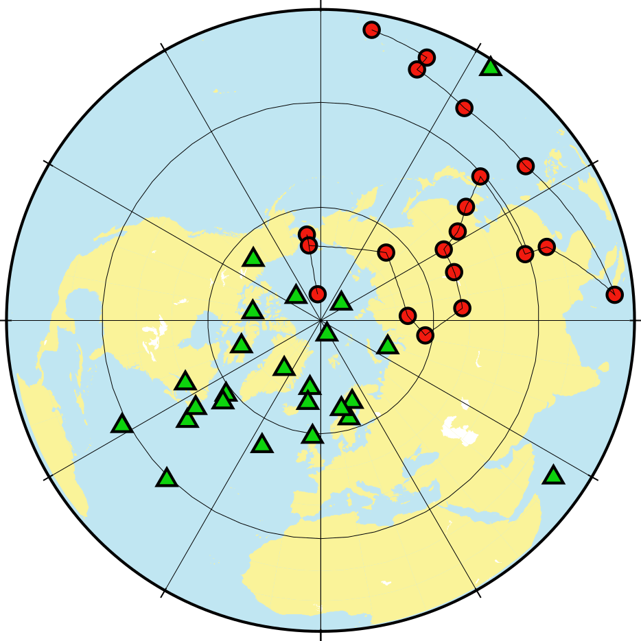
Figure 16.19:Circles are “reliable” mean poles from cratonic North America. (Data as listed in Voo (1990)). So-called “discordant poles” from western North America are plotted as triangles. [Data from Voo (1981).]
To illustrate this, we plot the data from North America that meet minimum V90 standards (). The mean poles from “cratonic” North America (from Voo (1990)) are plotted as circles in Figure 16.19 as well as so-called discordant paleomagnetic poles (from Voo (1981)). It is quite clear that the discordant poles do not fall anywhere near the APWP. Most are from western North America and indicate some clockwise rotations (the poles are rotated to the right of the expected poles). When taking into account the age of the formations, many also seem to have directions that are too shallow, which suggests possible northward transport of 1000s of kilometers. The validity and meaning of these discordant directions is still under debate, but it is obvious that most of the western Cordillera is not in situ.
16.7Inclination Only Data and APWPs
If a paleomagnetic data set comes from only vertically oriented cores, or if a particular region has undergone relative rotation with respect to the craton, the inclinations can still provide constraints on the APWP. Data from azimuthally un-oriented deep sea sediment cores were used by Tauxe et al. (1983) to help constrain the motion of the African plate during the Cenozoic and subsequent compilations have continued the practice (see, e.g., Besse & Courtillot (2002)). Voo (1992) used data from “mobile belts” that experienced relative rotation with respect to the craton to provide constraints on the Jurassic APWP of North America, a subject of some contention (see, e.g., Van Fossen & Kent (1990); Butler (1992); Van Fossen & Kent (1992); Van Fossen & Kent (1993)). We re-do the analysis for one specific time window (150 Ma) here as an example of the technique.
Use of inclination only data requires knowledge of the following:
The precise age of the rock unit under study: This is frequently constrained by magnetostratigraphy, biostratigraphy or radioisotopic data.
(Paleo-)vertical: Drill cores or “mobile belts” often are azimuthally unoriented but the direction to the (paleo-)vertical is known.
Cratonic affiliation: The allegiance of the rock unit under study to a particular continental fragment or craton must be known in order to rotate the site location into a common reference frame, for example “fixed South Africa”.
Data from at least three far-flung localities: One paleolatitude estimate (calculated from the inclination using the dipole formula in Chapter 2) defines a small circle path around the site location along which the paleopole must lie. Two such small circles may intersect at two points leaving the true paleopole position ambiguous. Three far flung locations will intersect at a unique point (see Figure 16.13). Additional data from fully constrained paleopole positions can be combined with the inclination only data for additional control.
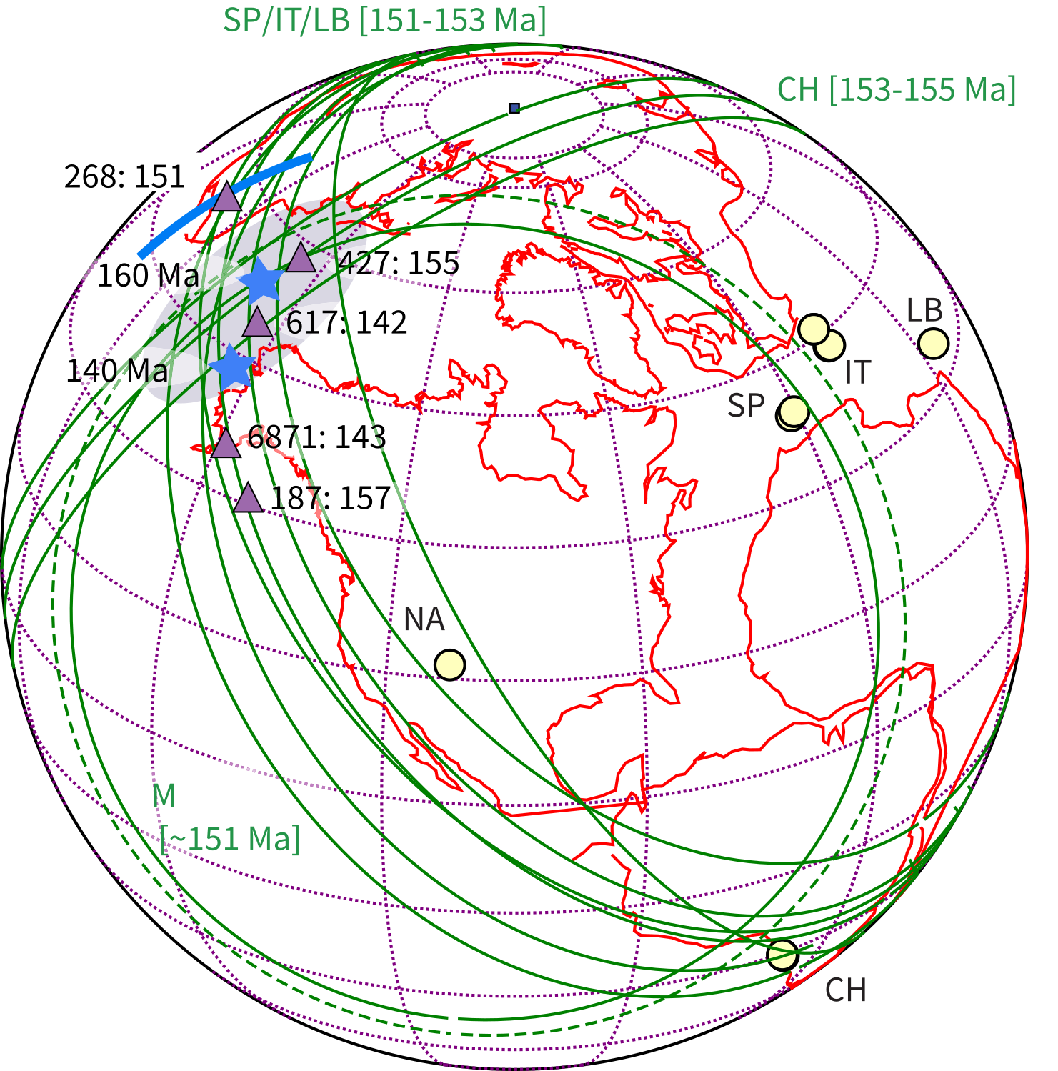
Figure 16.20:If local rotations are suspected for a given region, the inclination information can be converted to the equivalent paleo-colatitude small circles (green solid lines) on which the paleopole must lie. Site locations from ‘mobile regions’ are shown as open circles. LB: Lebanon, SP: Spain; IT: Italy; CH: Chile; NA: Morrison Formation on the Colorado Plateau of North America. Small circles (solid green lines) are the paleomagnetic colatitudes ( in Table 16.3) from inclination data. The dashed line is the paleolatitude from uncorrected inclination data of the Morrison Formation. Shaded ellipse indicates region of overlap among all small circles. Fully oriented poles are shown as purple triangles. Numbers are the GPMDB reference numbers followed by the age in Ma. See Table 16.3. All poles and observation sites have been rotated into South African coordinates for 155 Ma (see Section A.3.5.3) as have the continents. Pole number 268 is the Canelo Hills Volcanics from Arizona. If this region rotated about a vertical axis, the pole would lie along the solid blue line. Blue stars are the predicted poles of Besse & Courtillot (2002) in South African coordinates.
We mentioned earlier that May & Butler (1986) applied the PEP technique to paleomagnetic poles from North America (see Figure 16.11c), whereby the Jurassic poles (labelled “G”,“K”, etc. in the figure) were interpreted to fall along small circle segments generated by North American steady plate motion around several Euler poles. The steady motion, represented by the two tracks labelled “J1” and “J2” in the figure are separated by a “cusp” when the Euler pole shifted positions. May & Butler (1986) recognized the problem with the first-order interpretation of the data shown in Figure 16.11c noting that some of the poles may have come from portions of the North American continent that had suffered differential rotation (see Section 16.6) and they produced a second set of curves that assumed different amounts of rotation for different poles. Some poles may suffer from sedimentary inclination shallowing as well (see Chapter 7). In the end, the APWP must agree with all the “reliable” poles from the continent and the PEP version of the North American APWP did not agree with several poles from the North American continent considered highly reliable. It also disagreed with poles that had been rotated into North American coordinates (see, e.g., Van Fossen & Kent (1990)).
Table 16.3:Paleomagnetic data for Kimmeridgian.
| Name | Age (Ma) | Plate | (°N) | (°E) | Result/Ref. | ||||
|---|---|---|---|---|---|---|---|---|---|
| IK | 143 | NA | 42.5 | 283.5 | 58 | 203.1 | 271.3 | 35.5 | 6871/[1] |
| BL | 142 | EU | 4.3 | 74 | 74 | 183.1 | 264.9 | 49.2 | 617/[2] |
| Blue | 155 | EU | 47.3 | 7.2 | 77.2 | 149 | 263 | 58.1 | 427/[3] |
| SK | 157 | AF | -25.5 | 26.2 | 30.8 | 277.8 | 277.8 | 30.8 | 187/[4] |
| CH | 151 | NA | 31.5 | -110.5 | 62.2 | 130.3 | 10.0 | 306.0 | 268/[5] |
| Name | Age (Ma) | Plate | (°N) | (°E) | Ref. | ||||
|---|---|---|---|---|---|---|---|---|---|
| LB | 151-153 | AF | 34 | 34.75 | 34.0 | 34.8 | 27.7 | 75.3 | [6] |
| SG | 151-153 | IB:EU | 37.2 | 355.9 | 38.9 | 358.8 | 27.9 | 75.2 | [7] |
| C | 151-153 | IB:EU | 37.5 | 356.7 | 39.2 | 359.6 | 35.5 | 70.4 | [7] |
| AR | 145-153 | AF | 46 | 12 | 46.0 | 12.0 | 30.6 | 73.5 | [8] |
| GC | 145-149 | AF | 43.5 | 12.5 | 43.5 | 12.5 | 37.7 | 68.9 | [9] |
| V | 145-155 | AF | 43.5 | 12.75 | 43.5 | 12.8 | 31.3 | 73.1 | [9] |
| BG | 151-153 | AF | 46 | 12 | 46.0 | 12.0 | 45.3 | 63.2 | [10] |
| M | 148-151 | NA | 38 | -108 | 16.7 | 307.4 | 52.5 | 56.9 | [11] |
| M* | 148-151 | NA | 56.9 | 52.5 | [12] | ||||
| F | 155 | SA | -26.4 | -70.5 | -30.5 | 352.4 | -43.0 | 115 | [13] |
| LA | 153 | SA | -26 | -70.5 | -30.2 | 352.1 | -48.6 | 119.6 | [13] |
| LN | 155 | SA | -30.2 | 352.1 | -35.5 | 109.6 | [13] |
LB: Lebanese basalts; SG: Sierra Gorda; C: Carabuey (Kimm); AR: Upper Ammonitico Rosso; GC: Gorgo a Cerbara; V: Upper Valdorbia; BG: Bassano del Grappa; M: Morrison Fm; M*: Morrison Fm (E/I corrected); F: Flamenco dikes; LA: Las Animas dikes; LN: La Negra volcanics; IK: Ithaca kimberlites; BL: Berriasian limestones; Blue: Blue limestones; SK: Swartruggen kimberlites; CH: Canelo Hills Volcanics.
: Site location; : Site location rotated to fixed Africa (155 Ma finite rotation pole), IB used first the rotation to Europe of Rosenbaum et al. (2002); : average inclination; : paleomagnetic colatitude from .
References: [1] Van Fossen & Kent (1993); [2] Galbrun (1985); [3] Johnson et al. (1984); [4] Hargraves & Onstott (1980); [5] Kluth et al. (1982); [6] Gregor et al. (1974); Van Dongen et al. (1967); [7] Ogg et al. (1984); [8] Channell (1992); [9] Channell et al. (1984); [10] Vandenberg & Wonders (1976); [11] Steiner & Helsley (1975); [12] this book; [13] Randall & Taylor (1996).
: Pole latitude and longitude; : Pole location rotated to Africa (200 Ma finite rotation pole).
The Kimmeridgian poles listed in Table 16.3 are plotted as triangles on Figure 16.20 and are poorly clustered. We can augment the Kimmeridgian data set by allowing data from regions of possible local rotation with respect to the craton using the inclination only technique. There are many magnetostratigraphic data sets from the Jurassic spanning the Kimmeridgian from Italy Channell et al., 1984Channell, 1992Vandenberg & Wonders, 1976, Spain Ogg et al., 1984 and the Colorado Plateau Steiner & Helsley, 1975. Italy was once part of Africa, Spain is attached to Europe (after closing of the Bay of Biscay) and the Colorado Plateau is part of the North American continent. All are known or suspected to have experienced relative rotation with respect to their respective cratonic reference frames. In addition, there are data from igneous outcrops in Lebanon Gregor et al., 1974Van Dongen et al., 1967 and Chile Randall & Taylor, 1996 that have been dated as 150-155 Ma in age. Lebanon is part of Africa and Chile, part of South America. Note that we have not used the data of Irwin (1987) because the directions are indistinguishable from the present field and those from Forsythe & Chisholm (1994) because the normal and reverse data were not antipodal. There are a few poles available from stable regions with ages between 140 and 160 Ma, some of which were included in the compilation of Besse & Courtillot (2002). Details of the Jurassic data sets considered here are listed in Table 16.3.
The problem of possible inclination shallowing can be addressed with the so-called elongation/inclination correction method of Tauxe & Staudigel (2004) (see Section 16.4) and local rotations can be treated using the “inclination-only” method briefly described in Section 16.2. We focus here on the Kimmeridgian time interval ( 151-153 Ma) because there are quite a few paleomagnetic data available, albeit not all from volcanics in stable cratonic environments. Indeed, very few poles of this age are included in compilations such as Besse & Courtillot (2002) or Torsvik et al. (2008). We list five poles from the Global Paleomagnetic Data Base (GPMDB) with ages between 143 and 157 Ma. [NB: One of these is the “Canelo Hills” pole from Kluth et al. (1982) which was renamed the “Glance Conglomerate” by May & Butler (1986), labeled ‘G’ in Figure 16.11.]
The Morrison Formation is a classic ‘red-bed’ formation. Tuffs at the top and bottom of the formation have been dated by Kowallis et al. (1998) and range from 148 Ma to 151 Ma. Data from this formation have traditionally been divided into Upper and Lower Morrison means (UM and LM respectively in Figure 16.11b), but the short duration of the section suggests that it is unlikely to record significant plate motion and we have lumped all the data together here. Moreover, because the magnetization is thought to be carried by detrital hematite, notorious for inclination shallowing, we treated the data to the elongation/inclination test described in Section 16.4. The corrected inclination is steeper by about 4°, insignificantly different from the uncorrected inclination (see Table 16.3). The paleomagnetic colatitude derived from the uncorrected inclination is shown as the dashed line in Figure 16.20, labelled ‘M’.
The paleomagnetic poles from the ‘mobile’ regions must lie along the small circle tracks shown as green lines in Figure 16.20. Because there are inclination only data from three quite different regions, labelled CH, NA and SP/IT/LB, there is a unique crossing point within the shaded region where the paleopole must lie. This inclination only paleopole for the Kimmeridgian ( Ma) agrees well with the predicted paleopole from the synthetic APWP of Besse & Courtillot (2002). The fully determined poles (purple triangles) agree reasonably well with the inclination only data. Also note that if south eastern Arizona, home to the Canelo Hills pole (#268 in Figure 16.20) suffered rotation like the Colorado Plateau, the unrotated pole would lie along the heavy blue line in Figure 16.20, which does not improve the fit.
16.8Concluding Remarks
And so we return to where we started at the beginning of this book with an assumption that the geomagnetic field is essentially that of a centered dipole. There is no compelling evidence that the field has operated in a vastly different way in ancient times, apart from the puzzling change in reversal frequency. We are getting better at all aspects of paleomagnetic research from better designed field programs to better laboratory analyses to more sophisticated data analysis. There remains much to be done. Enjoy.
16.9Problems
Problem 1
a) Calculate the expected direction for about 20 Ma at a locality in the Mojave Desert (latitude of 34.5°N and longitude of 117.5°W). Use the function pmag.apwp( ) which is built on the Besse & Courtillot (2002) global apparent polar wander path to get the pole. Assume that the Mojave was on the North American Plate (which it was back then).
b) Go to the MagIC search interface at: http://
c) Fish out the data that are tilt corrected and make an equal area plot of all the directions. Use the usual functions ipmag.plot_net( ), ipmag.plot_di( ). Plot these in 5 million year color coded age groups. Put the expected direction on (both normal and reverse) as black stars. What do you think is going on?
Problem 2
Look back at the Problems for Chapter 15, and use the same data set. What tectonic plate is Site 522 on? Using the age range inferred from your magnetostratigraphic interpretation and knowing the plate and the present day location, find the appropriate paleopoles for the top (Oligo/Miocene boundary) and bottom (Eocene/Oligocene boundary) of the dataset from those of Besse & Courtillot (2002). Besse & Courtillot (2002) is what is implemented in the function pmag.apwp( ) to calculate the expected inclinations for the top and bottom 10 meters of the record, respectively. How do these inclinations compare with the ones in Site 522?
Problem 3
a) Find the appropriate pole of rotation from North America to South African coordinates for 90 Ma (use the right sign for the rotation angle!) from Section A.3.5.3. Or you can use the frp.get_pole( ) function in the pmagpy.frp module.
b) Use the function pmag.pt_rot( ) to transform the North American pole to South African coordinates using the method outlined in Section A.3.5.3. The North American pole for 90 Ma in BC02 is . The African pole is . How do your answers compare?
Problem 4
a) Go to the MagIC search interface at: http://
df.method_codes.unique( ).
You will notice that some have method codes of DE-DC2 (a DC code of 2, see Table 16.1) or even DC1! Filter for those with DC codes of 4 or 5 for the ‘best’ poles and concatenate them into a new DataFrame.
b) Some of the data come studies that have been superseded by later studies or the authors thought were ‘remagnetized’ or have been combined into other studies. You can see this looking at the ‘description’ column in the DataFrame. Exclude these studies by filtering on this column using the strings ‘emagnetiz’, ‘econdary’, ‘uperseded’, ‘synfolding’, ‘Data incl. in RESULT’, ‘verprint’. Also, there seem to be a lot of duplicate poles in our filter list. You can get rid of duplicates using the df.drop_duplicates method of Pandas.
c) Put the pole latitudes and longitudes into form that you can use with pmag.pt_rot( ) to rotate these to North American coordinates for 100 Ma. Get the poles of rotation from the frp.get_pole( ) function (or in Section A.3.5.3). You need to first rotate Europe to fixed African coordinates, then African to North American coordinates (you will have to change the sign of for the latter).
Compare your rotated pole with the synthetic pole of Besse & Courtillot (2002). You can find what this is by using the function pmag.apwp( ).
d) Make a plot of the continental configurations at 100 Ma using the function continents.get_continent in the pmagpy.continents module along with the pmagplotlib.plot_map( ) function. You will of course also need frp.get_pole( ) and pmag.pt_rot( ). Select the European, North American, African, South American, Indian, Australian and Antarctic continents.
- Hospers, J. (1955). Rock magnetism and polar wandering. Journal of Geology, 63(1), 59–74. 10.1086/626226
- Irving, E. (1958). Palaeogeographic reconstruction from palaeomagnetism. Geophysical Journal of the Royal Astronomical Society, 1(3), 224–237. 10.1111/j.1365-246X.1958.tb00056.x
- Irving, E. (1956). Palaeomagnetic and palaeoclimatological aspects of polar wandering. Geofisica Pura e Applicata, 33(1), 23–41. 10.1007/BF02629944
- Bird, P. (2003). An updated digital model of plate boundaries. Geochemistry, Geophysics, Geosystems, 4(3), 1027. 10.1029/2001GC000252
- DeMets, C., Gordon, R. G., Argus, D. F., & Stein, S. (1994). Effect of recent revisions to the geomagnetic reversal time scale on estimates of current plate motions. Geophysical Research Letters, 21(20), 2191–2194. 10.1029/94GL02118
- Bullard, E. C., Everett, J. E., & Smith, A. G. (1965). The fit of the continents around the Atlantic. Philosophical Transactions of the Royal Society of London A, 258(1088), 41–51. 10.1098/rsta.1965.0020
- Torsvik, T. H., & Cocks, L. R. M. (2017). Earth History and Palaeogeography. Cambridge University Press. 10.1017/9781316225523
- Torsvik, T. H., Van der Voo, R., Preeden, U., Mac Niocaill, C., Steinberger, B., Doubrovine, P. V., van Hinsbergen, D. J. J., Domeier, M., Gaina, C., Tohver, E., Meert, J. G., McCausland, P. J. A., & Cocks, L. R. M. (2012). Phanerozoic polar wander, palaeogeography and dynamics. Earth-Science Reviews, 114, 325–368. 10.1016/j.earscirev.2012.06.007
- Torsvik, T. H., Müller, R. D., Van der Voo, R., Steinberger, B., & Gaina, C. (2008). Global plate motion frames: Toward a unified model. Reviews of Geophysics, 46, RG3004. 10.1029/2007RG000227
- Halls, H. C. (1974). A paleomagnetic reversal in the Osler Volcanic Group, northern Lake Superior. Canadian Journal of Earth Sciences, 11(9), 1200–1207. 10.1139/e74-113
- Swanson-Hysell, N. L., Vaughan, A. A., Mustain, M. R., & Asp, K. E. (2014). Confirmation of progressive plate motion during the Midcontinent Rift’s early magmatic stage from the Osler Volcanic Group, Ontario, Canada. Geochemistry, Geophysics, Geosystems, 15(5), 2039–2047. 10.1002/2013GC005180
- Van der Voo, R. (1990). Phanerozoic paleomagnetic poles from Europe and North America and comparisons with continental reconstructions. Reviews of Geophysics, 28(2), 167–206. 10.1029/RG028i002p00167
- Besse, J., & Courtillot, V. (2002). Apparent and true polar wander and the geometry of the geomagnetic field over the last 200 Myr. Journal of Geophysical Research: Solid Earth, 107(B11), 2300. 10.1029/2000JB000050
- Butler, R. F. (1992). Paleomagnetism: Magnetic Domains to Geologic Terranes. Blackwell Scientific Publications.
- McElhinny, M. W., & McFadden, P. L. (2000). Paleomagnetism: Continents and Oceans (Vol. 73). Academic Press.