Chapter 5 and Chapter 7 discussed various hysteresis parameters and Chapter 11 and Chapter 12 developed the major features of paleomagnetic directional statistics. Here we go over some aspects in greater detail.
C.1Hysteresis Parameters
A typical hysteresis experiment involves determination of a hysteresis loop and frequently also a back-field curve (see Figure C.1). Processing of the data in the PmagPy software package (see, e.g., Example for hysteresis_magic.py) proceeds as follows:
Sometimes the descending and ascending hysteresis loops do not close because of instrument drift (see Figure C.1a). Ordinarily, the experiment should be re-done, but for small differences, we force the loops to close by subtracting the difference, interpolated from the maximum difference at the maximum field () to a zero difference at the minimum field ().
After closing the loops, we calculate the best-fit line to the data for the portion within 70% of , averaging data from both the ascending and descending loops. A difference in the absolute value of the y-intercepts for the ascending and descending loops indicates a vertical offset of the data, which is adjusted such that the two intercepts are equal. The average slope is the high-field susceptibility (), which is subtracted off. The data after these steps are shown as the dashed line in Figure C.1. The maximum magnetization after adjusting for the is the saturation magnetization .
Table C.1:Summary of hysteresis parameters.
| Symbol | Method | Section | Figure |
|---|---|---|---|
| high field susceptibility | Section 5.2.2 & Section 8.5 | Figure 5.5 & Figure C.1 | |
| saturation magnetization | Section 3.2.2 | Figure 5.5 & Figure C.1 | |
| saturation remanence | Section 5.2.1 & Section 7.7 | Figure 5.5 & Figure C.1 | |
| or | Coercivity | Paragraph & Section 5.2.1 | Figure 5.5 & Figure C.1 |
| Coercivity of remanence: | |||
| method | Section 5.2.1 | Figure C.1 | |
| ascending loop intercept method | Section 5.2.1 | Figure 5.5 | |
| Back-field method | Section 7.7 | Figure 7.21 & Figure C.1 | |
| method | Section 7.7 & Section 8.4.2 | Figure 7.21 & Figure 8.9 |
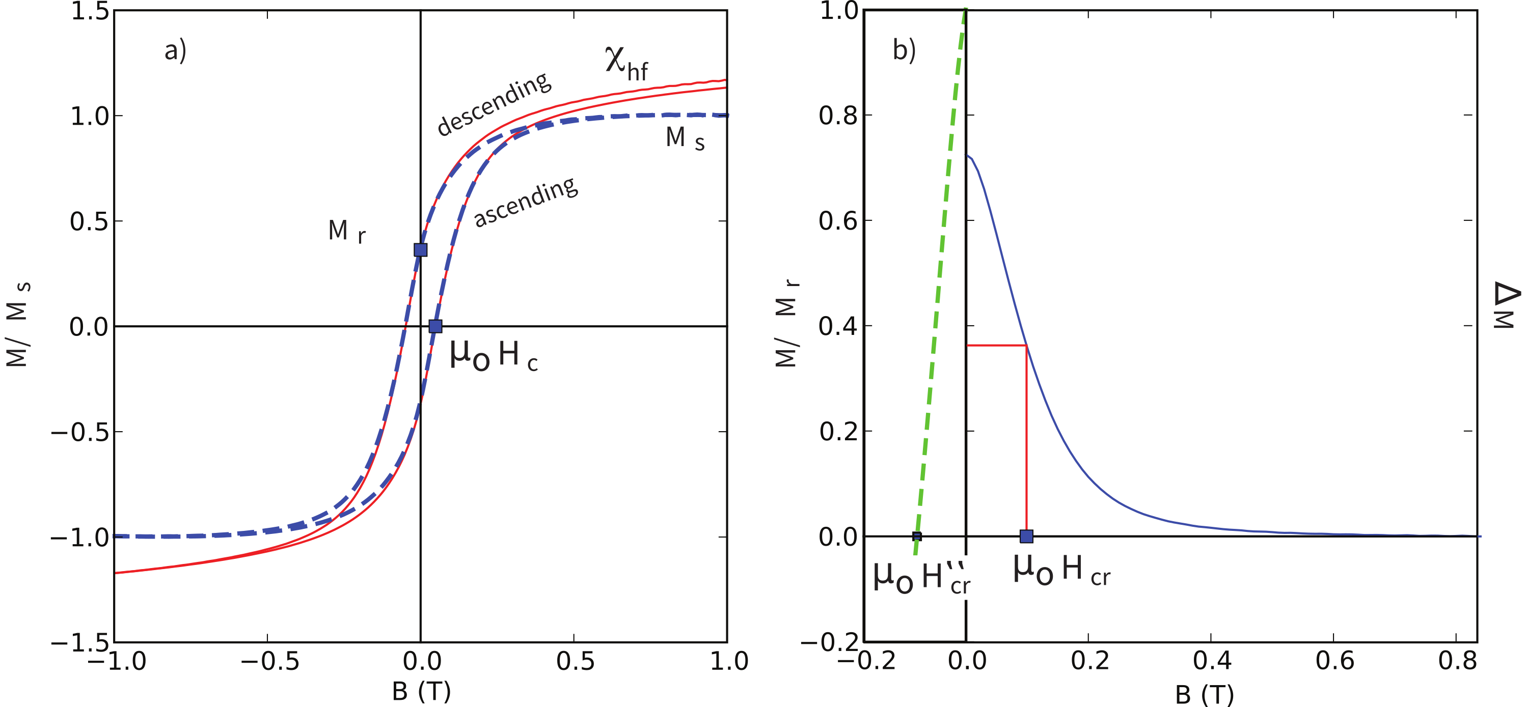
Figure C.1:Typical hysteresis experiment. a) Raw data are solid red line. Data are processed (see text) by closing the ascending and descending loops, subtracting the high field slope () and adjusting such that the y-intercepts are equal (that for the descending loop is labeled ). Processed data are dotted blue line. Coercivity () is the applied field for which a saturation magnetization () is reduced to zero. b) Difference between processed ascending and descending loops is the curve (solid blue line). Back-field IRM data shown normalized by saturation remanence () -- dashed green line. Two methods of estimating coercivity of remanence shown (see text).
Coercivity () is the field at which . We estimate this by finding the values of between which switches sign for both the ascending and descending loops (after adjustment), calculate a line and evaluate the for which . The coercivity is the average of the two estimates.
We fit a spline to the adjusted ascending and descending loops and resample the loops at even intervals of (usually 10 mT intervals). The curve shown in Figure C.1b is the difference between these two interpolated curves, averaging the data for negative and positive . The saturation remanence is the value of the curve at . The coercivity of remanence ( in Table C.1) is the field for which is half the value of . This is the “” method of coercivity of remanence calculation (see Chapter 5).
If there are “back-field” IRM data as in Figure C.1b, the coercivity of remanence can be estimated by finding (through interpolation) the applied field which reduces the saturation remanence () to zero. This is the “back field” method.
C.2Directional statistics
Table C.2:Critical values of for a random distribution Watson, 1956.
| 95% | 99% | 95% | 99% | ||
|---|---|---|---|---|---|
| 5 | 3.50 | 4.02 | 13 | 5.75 | 6.84 |
| 6 | 3.85 | 4.48 | 14 | 5.98 | 7.11 |
| 7 | 4.18 | 4.89 | 15 | 6.19 | 7.36 |
| 8 | 4.48 | 5.26 | 16 | 6.40 | 7.60 |
| 9 | 4.76 | 5.61 | 17 | 6.60 | 7.84 |
| 10 | 5.03 | 5.94 | 18 | 6.79 | 8.08 |
| 11 | 5.29 | 6.25 | 19 | 6.98 | 8.33 |
| 12 | 5.52 | 6.55 | 20 | 7.17 | 8.55 |
C.2.1Calculation of Watson’s 
Calculate , and where for the two data sets with samples using Equation 11.14 and Equation 11.16.
Calculate (where for the three axes) using Equation 11.15.
Calculate .
Find the weighted means for the two data sets:
Calculate the weighted overall resultant vector by
and the weighted sum by,
Finally, Watson’s is defined as
C.2.2Combining lines and planes
Calculate directed lines (two in our case) and great circles (one in our case) using principal component analysis (see Chapter 9) or Fisher statistics.
Assume that the primary direction of magnetization for the samples with great circles lies somewhere along the great circle path (i.e., within the plane).
Assume that the set of directed lines and unknown directions are drawn from a Fisher distribution.
Iteratively search along the great circle paths for directions that maximize the resultant vector for the directions.
Having found the set of directions that lie along their respective great circles, estimate the mean direction using Equation 11.15 and as:
The cone of 95% confidence about the mean is given by:
where and = .02
C.2.3Inclination only calculation
We wish to estimate the co-inclination () of Fisher distributed data (), the declinations of which are unknown. We define the estimated value of to be . McFadden & Reid (1982) showed that is the solution of:
which can be solved numerically.
They further define two parameters and as:
An unbiased approximation for the Fisher parameter , is given by:
The unbiased estimate of the true inclination is:
Finally, the is estimated by:
where is the critical value taken from the distribution (see F-distribution tables in statistics textbooks or online) with 1 and (-1) degrees of freedom.
C.2.4Kent 95% confidence ellipse
Kent parameters are calculated by rotating unimodal directions into the data coordinates by the transformation:
where , and the columns of are called the constrained eigenvectors of orientation matrix, (see Section A.3.5.4). The vector is parallel to the Fisher mean of the data, whereas and (the major and minor axes) diagonalize as much as possible subject to being constrained by (see Kent (1982), but note that his corresponds to in conventional paleomagnetic notation). The following parameters may then be computed:
As defined here, ( is closely approximated by the equation for in Chapter 11. Also to good approximation, and , where are the eigenvalues of the orientation matrix.
The semi-angles and subtended by the major and minor axes of the 95% confidence ellipse are given by:
where .
The tensor is, to a good approximation, equivalent to , the eigenvectors of the orientation matrix. Therefore, the eigenvectors of the orientation matrix give a good estimate for the directions of the semi-angles by:
where for example the component of the smallest eigenvector is denoted .
C.2.5Bingham 95% confidence parameters
The Bingham distribution is given by:
where and are as in the Kent distribution, are concentration parameters () and is a constant of normalization given by:
To estimate the axes of the Bingham confidence ellipse, we first calculate the eigenparameters of the orientation matrix as for Kent parameters and described in Section A.3.5.4 and Section C.2.4. The principal eigenvector of the orientation matrix is associated with the largest eigenvalue . In Bingham (1974), is the and is . In Bingham statistics, the direction is taken as the mean. Beware -- it is not always parallel to the Fisher mean of a unimodal set of directions.
The maximum likelihood estimates of , the concentration parameters are obtained by first maximizing the log likelihood function:
These are tabulated in Mardia & Zemroch (1977). Once these are estimated, the semi-axes of the 95% confidence ellipse around the mean direction are given by:
where is the value for significance ( for 95% confidence) with degrees of freedom and
Bingham (1974) set , so the semi axes of the confidence ellipse about the principal direction , associated with , are therefore:
and
Because , the semi-axes are positive numbers. Please note that here we use the corrected version of Tanaka (1999) as opposed to the more oft-quoted but erroneous treatment of Onstott (1980). Note also that the is required for because we have normalized the s to sum to unity for consistency with other eigenvalue problems in this book. The is missing in the treatment of Tanaka (1999) presumably because the eigenvalues sum to . Finally, note that these values of are in radians and must be converted to degrees for most applications.
C.3Paleointensity statistics
Paleointensity statistics have gotten somewhat out of hand of late. There are a bewildering variety of statistics that are used in the literature, with no consensus as to which ones are essential, which ones are helpful and which ones are irrelevant. This appendix will not help the reader in this regard, but merely attempts to assemble the ones we feel are the most useful.
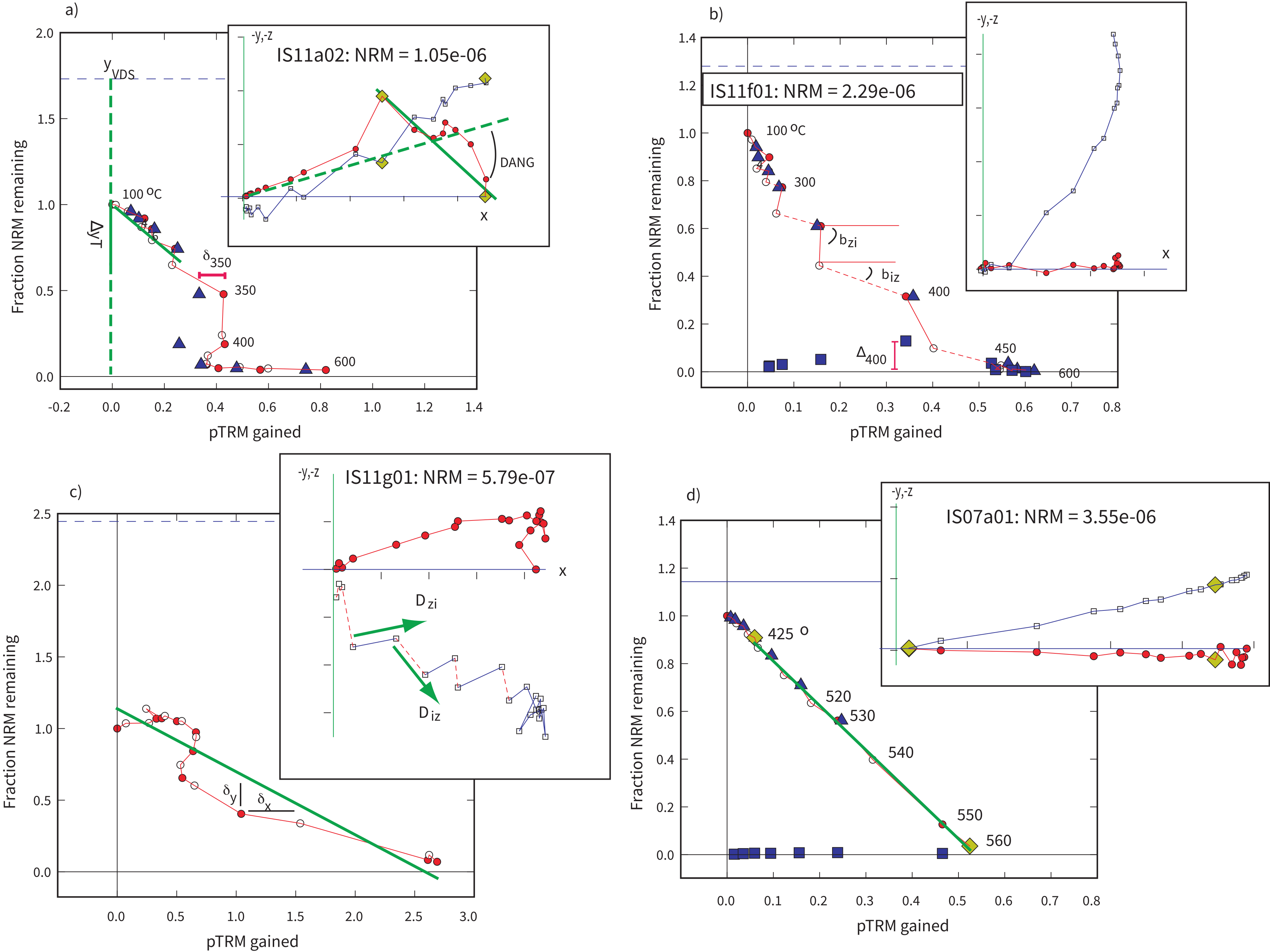
Figure C.2:Illustration of paleointensity parameters. Arai plots: The magnitude of the NRM remaining after each step is plotted versus the pTRM gained at each temperature step. Closed symbols are zero-field first followed by in-field steps (ZI) while open symbols are in-field first followed by zero field (IZ). Triangles are pTRM checks and squares are pTRM tail checks. Horizontal dashed lines are the vector difference sum (VDS) of the NRM steps. Vector endpoint plots: Insets are the x,y (solid symbols) and x,z (open symbols) projections of the (unoriented) natural remanence (zero field steps) as it evolves from the initial state (plus signs) to the demagnetized state. The laboratory field was applied along -Z. Diamonds indicate bounding steps for calculations. a) The is the fraction of the component used of the total VDS. The difference between the pTRM check and the original measurement at each step is . The inset shows the deviation angle (DANG) that a component of NRM makes with the origin. The maximum angle of deviation MAD is calculated from the scatter of the points about the best-fit line (solid green line). b) Data exhibit “zig-zag behavior” diagnostic for significant difference between blocking and unblocking temperatures. The Zig-zag for slopes compares slopes calculated between ZI and IZ steps () with those connecting IZ and ZI steps ). The difference between the pTRM tail check and the original measurement at each step is . c) reflects the scatter () about the best-fit slope (solid green line). The Zig-zag for directions compares those calculated between ZI and IZ steps () with those connecting IZ and ZI steps ). [Figures from Ben-Yosef et al. (2008).]
The Deviation of the ANGle (DANG; Tauxe & Staudigel (2004); see Chapter 9): The angle that the direction of the NRM component used in the slope calculations calculated as a best-fit line (see Section A.3.5.4) makes with the angle of the line anchoring the center of mass (see Section A.3.5.4) to the origin (see insert to Figure C.2a).
The Maximum Angle of Deviation (MAD; Kirschvink (1980); see Chapter 9): The scatter about the best-fit line through the NRM steps.
We can calculate the best-fit slope () for the data on the NRM-pTRM plot and its standard error (York (1966); Coe et al. (1978)). The procedure for calculating the best-fit slope, which is the best estimate for the paleofield, is given as follows:
a) Take the data points that span two temperature steps and , the best-fit slope relating the NRM () and the pTRM () data in a least squares sense (taking into account variations in both and ) is given by:
where is the average of all values and is the average of all values.
b) The y-intercept () is given by .
c) The standard error of the slope is:
The “scatter” parameter : the standard error of the slope (assuming uncertainty in both the pTRM and NRM data) over the absolute value of the best-fit slope (Coe et al. (1978)).
The remanence fraction, , was defined by Coe et al. (1978) as:
where is the length of the NRM segment used in the slope calculation (see Figure C.2).
The fraction of the total remanence (by vector difference sum), (Tauxe & Staudigel (2004)): While works well with single component magnetizations as in Figure C.2d where it reflects the fraction of the total NRM used in the slope calculation, it can be misleading when there are multiple components of remanence as in Figure C.2a. The values of for such specimens can be quite high, whereas the fraction of the total NRM is much less. We prefer to use a parameter which is the fraction of the total NRM, estimated by the vector difference sum (VDS; Chapter 9) of the entire zero field demagnetization data. The VDS (see Figure C.2a) “straightens out” the various components of the NRM by summing up the vector differences at each demagnetization step. is calculated as:
where is the vector difference sum of the entire NRM (see Figure C.2a and Chapter 9). This parameter becomes small, if the remanence is multi-component, whereas the original can be blind to multi-component remanences.
The Difference RATio Sum, DRATS: The difference between the original pTRM at a given temperature step (horizontal component of the circles in Figure C.2) and the pTRM check (horizontal component of the triangles in see Figure C.2), (see Figure C.2a), can result from experimental noise or from alteration during the experiment. Selkin & Tauxe (2000) normalized the maximum value within the region of interest by the length of the hypotenuse of the NRM/pTRM data used in the slope calculation. DRAT is therefore the maximum difference ratio expressed as a percentage. In many cases, it is useful to consider the trend of the pTRM checks as well as their maximum deviations. We follow Tauxe & Staudigel (2004) who used the sum of these differences. We normalize this difference sum by the pTRM acquired by cooling from the maximum temperature step used in the slope calculation to room temperature. This parameter is called the Difference RATio Sum or DRATS. Only pTRM checks at temperatures below the maximum bound are included in the DRATS calculation.
Maximum Difference % MD%: The absolute value of the difference between the original NRM measured at a given temperature step (vertical component of the circles in Figure C.2) and the second zero field step (known as the pTRM tail check) results from some of the pTRM imparted in the laboratory at having unblocking temperatures that are greater than . These differences (; see Figure C.2b) are plotted as squares. The Maximum Difference, normalized by the VDS of the NRM and expressed as a percentage is the parameter MD%.
Zig-Zag : In certain specimens, the IZZI protocol leads to rather interesting behavior, described in detail by Yu et al. (2004). The solid symbols in Figure C.2 are the zerofield-infield (ZI) steps and the intervening steps are the infield-zerofield (IZ) steps (open circles). Alternating the two results in a “zigzag” in some specimens. The zigzag can be in either the Arai diagrams (compare slope of solid versus dashed line segments in Figure C.2b) or in the orthogonal projections of the zero field vectors (compare directions of solid and dashed line segments in Figure C.2c). We therefore can define a parameter by testing the difference in either the two sets of slopes or the two sets of directions between the IZ steps and the ZI steps.
To test the significance of the difference between the zero-field IZ directions and those from the ZI zero-field steps, we calculate F-test () for Watson’s test for common mean (Watson (1983)). The zigzag for directions is ratio where is the critical value for at degrees of freedom (at the 95% level of confidence).
For the slopes, we calculate the mean and variance of the slopes for the IZ segments () and the ZI segments (). The parameter is the test for the two means. The zigzag for the slopes is the ratio where is critical value for with degrees of freedom (from a statistics table).
If the difference between the sets of directions and slopes is less than 2° or both and are less than unity, then . Otherwise is the larger of and .
The “gap factor” (Coe et al. (1978)) penalizes uneven distribution of data points and is:
where is given by:
and is the weighted mean of the gaps between the data points along the selected segment.
The Coe quality index combines the standard error of the slope, the NRM fraction and the gap factors by:
As data spacing becomes less uniform, decreases.
A quick and dirty test for the possibility of anisotropy of TRM is to compare the direction of the pTRM acquired in the laboratory field with the direction of the applied field. The angle between these two at the maximum pTRM temperature used in the slope calculation is defined here as . If this exceeds more than a few degrees, it is advisable to perform some sort of test for TRM (or ARM) anisotropy.
- Watson, G. S. (1956). A test for randomness of directions. Geophysical Supplements to the Monthly Notices of the Royal Astronomical Society, 7(4), 160–161. 10.1111/j.1365-246X.1956.tb05561.x
- McFadden, P. L., & Reid, A. B. (1982). Analysis of palaeomagnetic inclination data. Geophysical Journal of the Royal Astronomical Society, 69(2), 307–319. 10.1111/j.1365-246X.1982.tb04950.x
- Kent, J. T. (1982). The Fisher-Bingham distribution on the sphere. Journal of the Royal Statistical Society: Series B (Methodological), 44(1), 71–80. 10.1111/j.2517-6161.1982.tb01189.x
- Bingham, C. (1974). An antipodally symmetric distribution on the sphere. The Annals of Statistics, 2(6), 1201–1225. 10.1214/aos/1176342874
- Mardia, K. V., & Zemroch, P. J. (1977). Table of maximum likelihood estimates for the Bingham distribution. Journal of Statistical Computation and Simulation, 6, 29–34. 10.1080/00949657708810165
- Tanaka, H. (1999). Circular asymmetry of the paleomagnetic directions observed at low latitude volcanic sites. Earth, Planets and Space, 51(11), 1279–1286. 10.1186/BF03351604
- Onstott, T. C. (1980). Application of the Bingham distribution function in paleomagnetic studies. Journal of Geophysical Research: Solid Earth, 85(B3), 1500–1510. 10.1029/JB085iB03p01500
- Ben-Yosef, E., Ron, H., Tauxe, L., Agnon, A., Genevey, A., Levy, T. E., Avner, U., & Najjar, M. (2008). Application of copper slag in geomagnetic archaeointensity research. Journal of Geophysical Research: Solid Earth, 113(B8), B08101. 10.1029/2007JB005235
- Tauxe, L., & Staudigel, H. (2004). Strength of the geomagnetic field in the Cretaceous Normal Superchron: New data from submarine basaltic glass of the Troodos Ophiolite. Geochemistry, Geophysics, Geosystems, 5(2), Q02H06. 10.1029/2003GC000635
- Kirschvink, J. L. (1980). The least-squares line and plane and the analysis of palaeomagnetic data. Geophysical Journal International, 62(3), 699–718. 10.1111/j.1365-246X.1980.tb02601.x
- York, D. (1966). Least-squares fitting of a straight line. Canadian Journal of Physics, 44(5), 1079–1086. 10.1139/p66-090
- Coe, R. S., Grommé, S., & Mankinen, E. A. (1978). Geomagnetic paleointensities from radiocarbon-dated lava flows on Hawaii and the question of the Pacific nondipole low. Journal of Geophysical Research, 83(B4), 1740–1756. 10.1029/JB083iB04p01740
- Selkin, P. A., & Tauxe, L. (2000). Long-term variations in palaeointensity. Philosophical Transactions of the Royal Society of London A, 358(1768), 1065–1088. 10.1098/rsta.2000.0574
- Yu, Y., Tauxe, L., & Genevey, A. (2004). Toward an optimal geomagnetic field intensity determination technique. Geochemistry, Geophysics, Geosystems, 5(2), Q02H07. 10.1029/2003GC000630
- Watson, G. S. (1983). Statistics on Spheres (Vol. 6). Wiley-Interscience.