Rocks often contain assemblages of ferromagnetic minerals dispersed within a matrix of diamagnetic and paramagnetic minerals. In later chapters, we will be concerned with the magnetization of these assemblages, but here we continue our investigation of the behavior of individual particles. In Chapter 3, we learned that in some crystals electronic spins work in concert to create a spontaneous magnetization that remains in the absence of an external field. The basis of paleomagnetism is that these ferromagnetic particles carry the record of ancient magnetic fields. What allows the magnetic moments to come into equilibrium with the geomagnetic field and then what fixes that equilibrium magnetization into the rock so that we may measure it millions or even billions of years later? We will begin to answer these questions over the next few chapters.
We will start with the second part of the question: what fixes magnetizations in particular directions? A basic principle is that ferromagnetic particles have various contributions to the magnetic energy which controls their magnetization. No matter how simple or complex the combination of energies may become, the grain will seek the configuration of magnetization which minimizes its total energy. The short answer to our question is that certain directions within magnetic crystals are at lower energy than others. To shift the magnetization from one “easy” direction to another requires energy. If the barrier is high enough, the particle will stay magnetized in the same direction for a very long time—say, billions of years. In this chapter, we will address the causes and some of the consequences of these energy barriers for the magnetization of rocks. Note that in this chapter we will be dealing primarily with energy densities (volume normalized energies) as opposed to energy. We will distinguish the two by the convention that energies are given with the symbol and energy densities with .
In Chapter 6, we will discuss the behavior of common magnetic minerals, but to develop the general theory, it is easiest to focus on a single mineral. We choose here magnetite Figure 4.1, as it has a simple cubic structure and has been the subject of intensive study. However, we will occasionally introduce concepts appropriate for other magnetic minerals when it will be informative.
![Three-panel figure: (a) photo of a dark, lustrous magnetite octahedron, (b) ball-and-stick model of the cubic inverse spinel crystal structure with oxygen anions and iron cations on tetrahedral and octahedral sites, (c) 3D anisotropy energy surface with lobes along hard [100] axes and dimples along easy [111] axes.](/Essentials-JupyterBook/build/magnetite-96fc00df1ecfa50ccecfa6a850a91974.png)
Figure 4.1:a) A magnetite octahedron. [Photo of Lou Perloff in The Photo-Atlas of Minerals.] b) Internal crystal structure. Directions of the body diagonal ([111] direction) and orthogonal to the cubic faces ([001] direction) are shown as arrows. Big red dots are the oxygen anions. The blue dots are iron cations in octahedral coordination and the yellow dots are in tetrahedral coordination. Fe sits on the A sites and Fe and Fe sit on the B sites. c) Magnetocrystalline anisotropy energy as a function of direction within a magnetite crystal at room temperature. The easiest direction to magnetize (the direction with the lowest energy — note dimples in energy surface) is along the body diagonal (the [111] direction). [Figure from Williams & Dunlop (1995).]
The simplest permanently magnetized particles are uniformly magnetized and are called single domain (SD). It is only in the smallest grains that such parallel alignment of spins is the lowest energy state. As particles get larger, the energy landscape changes and energy is minimized by spins curling around within a grain to form a vortex. This vortex state can be stable and long-lived and have behavior similar to single-domain grains which has led to such grains being referred to as pseudo-single domain (PSD). In grains that are larger still, spins organize themselves into regions with quasi-uniform magnetization (magnetic domains) separated by domain walls and are called multidomain (MD) particles. These more complicated spin structures are challenging to model and most paleomagnetic theory is based on single domain behavior. Therefore, we begin with a discussion of the energies of uniformly magnetized (single-domain) particles.
4.1The magnetic energy of particles
4.1.1Exchange energy
We learned in Chapter 3 that some crystalline states are capable of ferromagnetic behavior because of quantum mechanical considerations. Electrons in neighboring orbitals in certain crystals “know” about each other’s spin states. In order to avoid sharing the same orbital with the same spin (hence having the same quantum numbers — not allowed by Pauli’s exclusion principle), electronic spins in such crystals act in a coordinated fashion. They will be either aligned parallel or antiparallel according to the details of the interaction. This exchange energy density () is the source of spontaneous magnetization and is given for a pair of spins by:
where is the exchange integral and and are spin vectors. Depending on the details of the crystal structure (which determines the size and sign of the exchange integral), exchange energy is at a minimum when electronic spins are aligned parallel or anti-parallel.
We define here a parameter that we will use later: the exchange constant where is the interatomic spacing. = 1.33 × 10 Jm for magnetite, a common magnetic mineral.
Recalling the discussion in Chapter 3, while orbitals are spherical, the electronic orbitals “poke” in certain directions. Hence spins in some directions within crystals will be easier to coordinate than in others. We can illustrate this using the example of magnetite, a common magnetic mineral (Figure 4.1a). Magnetite octahedra (Figure 4.1a), when viewed at the atomic level (Figure 4.1b) are composed of one ferrous (Fe) cation, two ferric (Fe) cations and four O anions. Each oxygen anion shares an electron with two neighboring cations in a covalent bond.
In Chapter 3, we mentioned that in some crystals, spins are aligned anti-parallel, yet there is still a net magnetization, a phenomenon we called ferrimagnetism. This can arise from the fact that not all cations have the same number of unpaired spins. Magnetite, with its ferrous (4 ) and ferric (5 ) states is a good example. There are three iron cations in a magnetite crystal giving a total of 14 to play with. Magnetite is very magnetic, but not that magnetic! From Figure 4.1b we see that the ferric ions all sit on the tetrahedral (A) lattice sites and there are equal numbers of ferrous and ferric ions sitting on the octahedral (B) lattice sites. The unpaired spins of the cations in the A and B lattice sites are aligned anti-parallel to one another because of superexchange (Chapter 3) so we have 9 on the B sites minus 5 on the A sites for a total of 4 per unit cell of magnetite.
4.1.2Magnetic moments and external fields
We know from experience that there are energies associated with magnetic fields. Just as a mass has a potential energy when it is placed in the gravitational field of another mass, a magnetic moment has an energy when it is placed in a magnetic field. This energy has many names (magnetic energy, magnetostatic energy, Zeeman energy, etc.). Here we will work with the volume normalized magnetostatic interaction energy density (). This energy density essentially represents the interaction between the magnetic lines of flux and the magnetic moments of the electronic spins. It is energy that aligns magnetic compass needles with the ambient magnetic field. We find the volume-normalized form (in units of J m) by noting that magnetization is moment per unit volume, (see Chapter 1)::
is at a minimum when is aligned with , so the magnetostatic energy acts to rotate the magnetization toward the applied field. Single-domain particles have a quasi-uniform magnetization and the application of a magnetic field does not change the net magnetization, which remains at saturation (). Although the magnetostatic energy favors alignment with the applied field, the magnetizations in many particles do not rotate freely (or we would not have paleomagnetism!). There is another contribution to the energy of the magnetic particle associated with the magnetic crystal itself. This energy depends on the direction of magnetization in the crystal — it is anisotropic — and is called anisotropy energy. Anisotropy energy creates barriers to free rotation of the magnetization within the magnetic crystal, which lead to energetically preferred directions for the magnetization within individual single-domain grains.
There are many causes of anisotropy energy. The most important ones derive from the details of crystal structure (magnetocrystalline anisotropy energy), the state of stress within the particle (magnetostriction), and the shape of the particle, (shape anisotropy). We will consider these briefly in the following subsections.
4.1.3Magnetocrystalline anisotropy energy
For equant single-domain particles or particles with low saturation magnetizations, the crystal structure dominates the magnetic energy. The so-called easy directions of magnetization are crystallographic directions along which magnetocrystalline energy is at a minimum.
For a cubic crystal like magnetite at room temperature, the magnetocrystalline anisotropy energy density is expressed in terms of the direction cosines — the cosines of the angles between the magnetization direction and the crystallographic axes [100], [010], [001] (see Section A.3.5.1 for review of direction cosines):
where and are empirically determined magnetocrystalline anisotropy constants with units of Jm (so is an energy density). Magnetite (cubic above 120 K) has = −1.35 × 10 Jm at room temperature. The result of this equation with these constants is that the easy directions are along the [111] body diagonals and the hard directions are along [100]. The interactive visualization below lets you explore this energy surface in 3D: the bulges along the hard [100] directions (red axes) and the dimples along the easy [111] directions (blue dashed axes) are a direct result of of (4.3). The energy is minimized along the [111] body diagonals with energy barriers between them due to the hard directions. Toggle between “Energy Landscape” and “Crystal Geometry” to compare the energy surface with the physical cubic crystal geometry.
As a consequence of the magnetocrystalline anisotropy energy, once the magnetization is aligned with an easy direction, work must be done to change it. In order to switch from one easy axis to another (e.g. from one direction along the body diagonal to the opposite for cubic magnetite), the magnetization has to traverse a path over an energy barrier which is the difference between the energy in the easy direction and that in the intervening hard direction. In the case of magnetite at room temperature, this energy barrier is (for )
4.1.3.1Temperature dependence of anisotropy
Because electronic interactions depend heavily on interatomic spacing, magnetocrystalline anisotropy constants are a strong function of temperature. The effect of this is dramatic in magnetite with progressively changing until it becomes zero at 130 K — this temperature is known as the isotropic point (Figure 4.2).
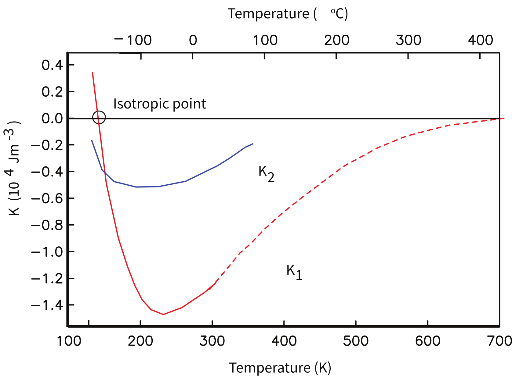
Figure 4.2:Variation of and of magnetite as a function of temperature. Solid lines are data from Syono & Ishikawa (1963). Dashed lines are data from Fletcher & O'Reilly (1974).
Given that at the isotropic point, there is minimal magnetocrystalline anisotropy at 130 K. The large energy barriers that act to keep the magnetizations parallel to the body diagonal are gone and the spins can wander more freely through the crystal. The interactive visualization below shows the energy landscape at 130 K, where the anisotropy energy is nearly uniform in all directions.
The change in magnetocrystalline anisotropy at low temperature can have a profound effect on the magnetization. As temperature decreases from room temperature, passes through zero at about 130 K — the isotropic point (). Below the isotropic point, the energy barriers rise again, but with a different topology: the cube axes become the energy minima and the body diagonals become the high energy directions — the reverse of the room-temperature situation. At still lower temperature (~120 K), the crystal structure of magnetite distorts from cubic to monoclinic at the Verwey temperature (). This distortion is driven by charge ordering: above , the extra electron shared between Fe²⁺ and Fe³⁺ on the octahedral lattice sites hops rapidly, making the sites equivalent; below , the charges localize into an ordered arrangement of Fe²⁺ and Fe³⁺, and the size difference between these ions distorts the lattice.
The combined effect of these transitions on magnetization is illustrated in Figure 4.3, which shows the remanence of a sample magnetized to saturation at room temperature, then cooled to low temperature and rewarmed. On cooling, the magnetization progressively decreases through the isotropic point — where the anisotropy momentarily drops to zero and the easy axes switch — and drops further through the Verwey transition where the crystal structure changes. On rewarming, only partial recovery occurs. This is the basis for low-temperature demagnetization (LTD). The remanence loss is predominantly a multidomain effect: loosely pinned domain walls reorganize as the anisotropy changes and do not all return to their original positions on rewarming. The portion that survives — the low-temperature memory — includes the remanence of single-domain grains (which are largely unaffected by LTD) as well as remanence held by strongly pinned domain walls in larger grains.
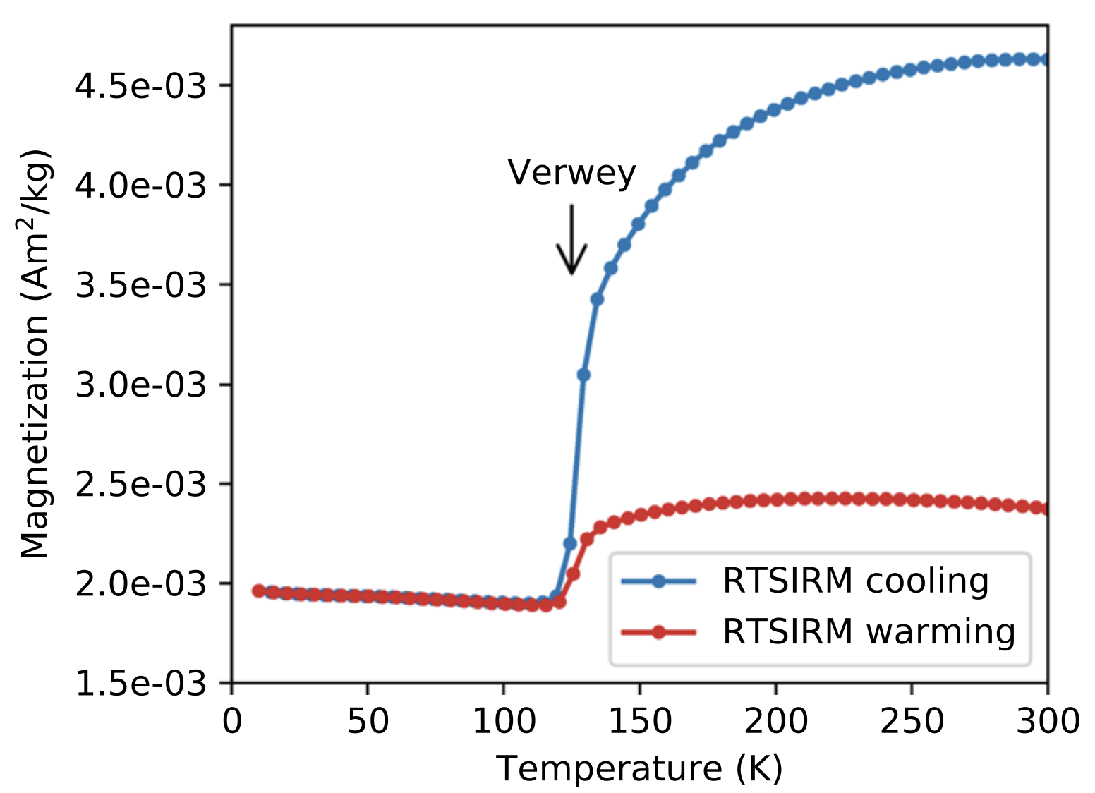
Figure 4.3:The magnetization of magnetite-bearing basaltic dike specimen that was given a saturating isothermal remanent magnetization at room temperature (RTSIRM) before being cooled to 10 K and warmed back up to 300 K. On cooling, the magnetization decreases through the isotropic point (~130 K) and drops sharply at the Verwey transition (~120 K). On rewarming, only partial recovery occurs — the difference is the multidomain remanence lost during LTD. Data from Swanson-Hysell et al. (2021) available in the MagIC database https://
4.1.3.2Uniaxial magnetocrystalline anisotropy
Cubic symmetry (as in the case of magnetite) is just one of many types of crystal symmetries. Another important form is uniaxial symmetry which can arise from crystal shape or structure. The energy density for uniaxial magnetic anisotropy is:
Here the magnetocrystalline constants have been designated to distinguish them from used before. When , the symmetry axis itself is the easy direction — an easy axis. When is negative, the symmetry axis is energetically unfavorable and the magnetization is confined to the plane perpendicular to it — an easy plane.
An example of a mineral dominated by uniaxial anisotropy is hematite. The magnetization of hematite is complicated, as we shall learn in Chapter 6 and Chapter 7, but one source of magnetization is spin-canting (see Chapter 3) within the basal plane. The uniaxial anisotropy perpendicular to the basal plane is very strong (), confining the magnetization to the easy plane. Within the basal plane, the anisotropy is orders of magnitude weaker so the magnetization theoretically wanders fairly freely. In reality, stress anisotropy from defects and internal strain (see next section) pins the magnetization direction within the basal plane much more effectively than magnetocrystalline anisotropy alone would predict.
The interactive visualization below demonstrates the energy landscape for hematite’s uniaxial anisotropy. The perpendicular anisotropy constant is K₁ = -1.2 × 10⁶ J/m³ Dunlop & Özdemir (1997), while the in-plane anisotropy is much weaker at 0-13 J/m³ Martı́n-Hernández & Guerrero-Suárez (2012). The energy surface shows high energy along the c-axis (hard direction) and low energy in the basal plane (easy directions).
4.1.4Magnetostriction — stress anisotropy
Exchange energy depends strongly on the details of the physical interaction between orbitals in neighboring atoms with respect to one another, hence changing the positions of these atoms will affect that interaction. Put another way, straining a crystal will alter its magnetic behavior. Similarly, changes in the magnetization can change the shape of the crystal by altering the shapes of the orbitals. This is the phenomenon of magnetostriction. The magnetic energy density caused by the application of stress to a crystal can be approximated by:
where is an experimentally derived constant, is the stress, and is the angle of the stress with respect to the crystallographic axis. Moskowitz (1993) measured the magnetostriction constants parallel to [111] and [100] in magnetite and found and to be and , respectively. is given by:
so for magnetite is about 38 × 10. Stress has units of Nm which have the same fundamental units as Jm, so is dimensionless. Note the similarity in form of magnetostriction and uniaxial anisotropy giving rise to a single “easy axis” within the crystal.
4.1.5Magnetostatic (shape) anisotropy
There is one more important source of magnetic anisotropy: shape. To understand how crystal shape controls magnetic energy, we need to understand the concept of the internal demagnetizing field of a magnetized body. In Figure 4.4a we show the magnetic vectors within a ferromagnetic crystal. These produce a magnetic field external to the crystal that is proportional to the magnetic moment (see Chapter 1). This external field is identical to a field produced by a set of free poles distributed over the surface of the crystal (Figure 4.4b). The surface poles do not just produce the external field, they also produce an internal field shown in Figure 4.4c. The internal field is known as the demagnetizing field (). is proportional to the magnetization of the body and is sensitive to the shape. For a simple sphere in Figure 4.4a and applied field condition shown in Figure 4.4d, the demagnetizing field is given by:
where is a demagnetizing factor determined by the shape. In fact, the demagnetizing factor depends on the orientation of within the crystal and therefore is a tensor (see Section A.3.5 for review of tensors). The more general equation is where and are vectors and is a 3 × 3 tensor. For now, we will simplify things by considering the isotropic case of a sphere in which reduces to the single value scalar quantity .
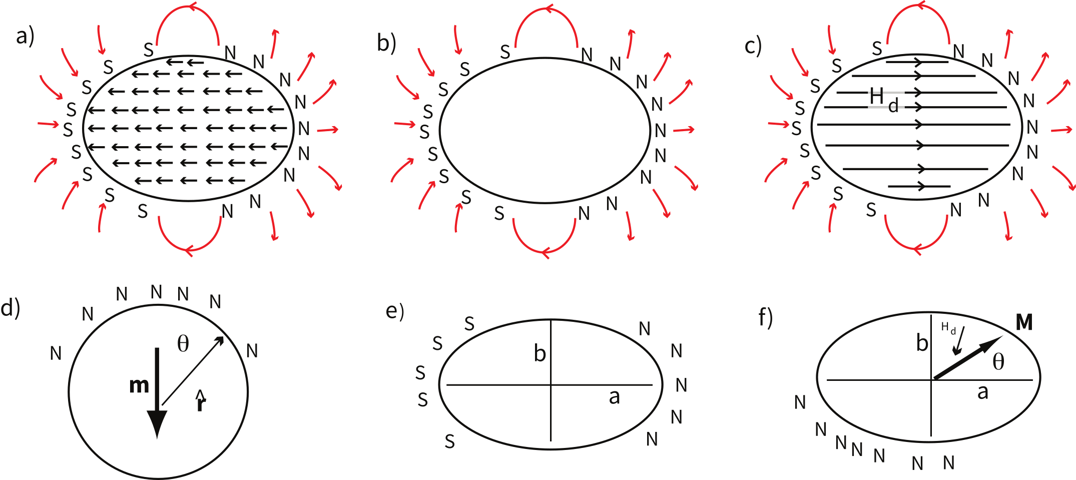
Figure 4.4:a) Internal magnetizations within a ferromagnetic crystal. b) Generation of an identical external field from a series of surface monopoles. c) The internal “demagnetizing” field resulting from the surface monopoles. [Redrawn from O'Reilly (1984).] d) Surface monopoles on a sphere. e) Surface monopoles on an ellipse, with the magnetization parallel to the elongation. f) Demagnetizing field resulting from magnetization at angle from axis in prolate ellipsoid.
For a sphere, the surface poles are distributed over the surface such that there are none at the “equator” and most at the “pole” (see Figure 4.4d). Potential field theory shows that the external field of a uniformly magnetized body is identical to that of a centered dipole moment of magnitude (where is volume). At the equator of the sphere as elsewhere, . But the external field at the equator is equal to the demagnetizing field just inside the body because the field is continuous across the body. We can find the equatorial (tangential) demagnetizing field at the equator by substituting in the equatorial colatitude into from Chapter 1, so:
Using the fact that magnetization (in units of Am) is the moment (in units of Am) per unit volume (in units of m) and the volume of a sphere is , we have:
so substituting and solving for we get , hence .
Different directions within a non-spherical crystal will have different distributions of free poles (see Figure 4.4e,f). In fact, the surface density of free poles is given by . Because the surface pole density depends on the direction of magnetization, so too will . In the case of a prolate ellipsoid magnetized parallel to the elongation axis (Figure 4.4e), the free poles are farther apart than across the grain, hence, intuitively, the demagnetizing field, which depends on , must be less than in the case of a sphere. Thus, . Similarly, if the ellipsoid is magnetized along (Figure 4.4e), the demagnetizing field is stronger or .
Getting back to the magnetostatic energy density, , remember that includes both the external field and the internal demagnetizing field . Therefore, magnetostatic energy density from both the external and internal fields is given by:
The two terms in Equation 4.10 are the by now familiar magnetostatic energy density , and the magnetostatic self energy density or the demagnetizing energy density . can be estimated by “building” a magnetic particle and considering the potential energy gained by each incremental volume as it is brought in () and integrating. The appears in order to avoid counting each volume element twice and the disappears because all the energies we have been discussing are energy densities — the energy per unit volume.
For the case of a uniformly magnetized sphere, we get back to the relation and simplifies to:
In the more general case of a prolate ellipsoid, can be represented by the two components parallel to the and axes (see Figure 4.4f) with unit vectors parallel to them . So, . Each component of has an associated demagnetizing field where are the eigenvalues of the tensor (the values of the demagnetizing tensor along the principal axes and ). In this case, the demagnetizing energy can be written as:
In an ellipsoid with three unequal axes , (in SI; in cgs units the sum is 4). For a long needle-like particle, and . A useful approximation for nearly spherical particles is Stacey & Banerjee (1974). For more spheroids, see Nagata (1961) (p. 70) and for the general case, see Dunlop & Özdemir (1997). In the absence of an external field, the magnetization will be parallel to the long axis () and the magnetostatic energy density (also known as the ‘self’ energy) is given by:
Note that the demagnetizing energy in Equation 4.12 has a uniaxial form, directionally dependent only on , with the constant of uniaxial anisotropy . is the difference between the largest and smallest values of the demagnetizing tensor .
For a prolate ellipsoid and choosing for example we find that . The magnetization of magnetite is 480 kAm, so 2.7 × 10 Jm. This is somewhat larger than the absolute value of for magnetocrystalline anisotropy in magnetite (= −1.35 × 10 Jm), so the magnetization for even slightly elongate grains will be dominated by uniaxial anisotropy controlled by shape. Minerals with low saturation magnetizations (like hematite) will not be prone to shape dominated magnetic anisotropy, however.
4.1.6Magnetic energy and magnetic stability
Paleomagnetists worry about how long a magnetization can remain fixed within a particle and we will begin to discuss this issue later in the chapter. It is worth pointing out here that any discussion of magnetic stability will involve magnetic anisotropy energy because this controls the energy required to change a magnetic moment from one easy axis to another. One way to accomplish this change is to apply a magnetic field sufficiently large that its magnetic energy exceeds the anisotropy energy. The magnetic field capable of flipping the magnetization of an individual uniformly magnetized particle (at saturation, or ) over the magnetic anisotropy energy barrier is the microscopic coercivity . For uniaxial anisotropy () and for cubic magnetocrystalline anisotropy (), microscopic coercivity is given by:
respectively (see Dunlop & Özdemir (1997) for a more complete derivation). For elongate particles dominated by shape anisotropy, reduces to . [Note that the units for coercivity as derived here are in Am, although they are often measured using instruments calibrated in tesla. Technically, because the field doing the flipping is inside the magnetic particle and (measured in tesla) depends on the magnetization as well as the field , coercivity should be written as if the units are quoted in tesla.] Microscopic coercivity is another parameter with many names: flipping field, switching field, intrinsic coercivity and also more loosely, the coercive field and coercivity. We will come back to the topic of coercivity in Chapter 5.
4.2Magnetic domains
So far we have been discussing hypothetical magnetic particles that are uniformly magnetized. Particles with strong magnetizations (like magnetite) have self energies that quickly become quite large because of the dependence on the square of the magnetization. We have been learning about several mechanisms that tend to align magnetic spins. In very small particles of magnetite (less than 60 nm for equant grains Nagy et al. (2017)), exchange energy dominates and the spins are uniformly aligned — the particle is single domain (SD). In larger particles, the self energy increasingly competes with the exchange and magnetocrystalline energies, and crystals develop distinctly non-uniform states of magnetization.
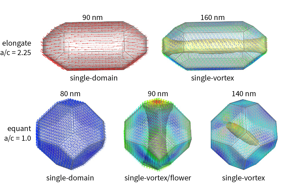
Figure 4.5:Micromagnetic simulations of remanent domain states in magnetite computed using MERRILL Williams et al., 2024. The elongate particles have an aspect ratio (b/a) of 2.25 while the equant particles are equidimensional. The numbers above the grains correspond to the equivalent spherical volume diameters (which is effectively the diameter for the equant ones; and a way to succinctly summarize the grain length for the elongate ones). The arrows show local magnetization direction while the colors indicate alignment with magnetocrystalline easy axes. For the elongate grains, the 90 nm grain has single-domain behavoir while the 160 nm grain has a vortex aligned with the long axis (which is the easy axis). The 80 nm equant grain is in a single-domain state, while the 90 nm grain is in an intermediate flower state with the initiation of a vortex. At a size of 140 nm there is a vortex aligned with the crystallographic easy axis. [From Williams et al. (2024).]
There are multiple strategies for magnetic particles to reduce self energy. Numerical models (called micromagnetic models) can find internal magnetization configurations that minimize the energies discussed in the preceding sections. Modern micromagnetic codes such as MERRILL Ó Conbhuí et al., 2018 allow us to peer into the state of magnetization inside magnetic particles. Figure 4.5 shows the progression of remanent states as particle size increases, computed using MERRILL Williams et al., 2024. In the smallest grains, the exchange energy overwhelms the self energy and the magnetization is nearly uniform — the SD state. As equant grains grow beyond about 60 nm, the self energy becomes large enough to perturb the magnetization near particle surfaces, causing spins at the edges to splay outward while the interior remains broadly aligned. This is the flower state (Figure 4.5e), so named because the fanning spins at the surface resemble the opening of a flower. By about 80 nm, the self energy is large enough that the magnetization curls into a closed loop, forming a vortex state (Figure 4.5b,c,f) with a narrow core of spins Nagy et al., 2017. The net remanent moment of a vortex particle is carried almost entirely by this core, since the curling spins surrounding it largely cancel. In elongated grains, shape anisotropy aligns both the vortex core and the overall remanence along the long axis of the particle (Figure 4.5a–c). The curling magnetization dramatically reduces the external field of the particle (and hence its self energy), while the exchange energy cost remains modest because neighboring spins change direction only gradually. In the smallest particles, the spins would have to curl too tightly and the exchange energy cost keeps them uniformly magnetized in the SD state. Particles with vortex cores share many properties of SD grains — in particular, they can carry extremely stable magnetic remanence with relaxation times exceeding the age of the Solar System Nagy et al., 2017 — which has led to them being termed pseudo-single domain (PSD) particles.
As particles grow larger (>~200 nm), they break into multiple magnetic domains, separated by narrow zones of rapidly changing spin directions called domain walls. Magnetic domains can take many forms. We illustrate a few in Figure 4.6. The uniform case (single domain) is shown in Figure 4.6a. The external field is very large because the free poles are far apart (at opposite ends of the particle). When the particle organizes itself into two domains (Figure 4.6b), the external field is reduced by about a factor of two. In the case of four lamellar domains (Figure 4.6c), the external field is quite small. The introduction of closure domains as in Figure 4.6d reduces the external field to nothing.
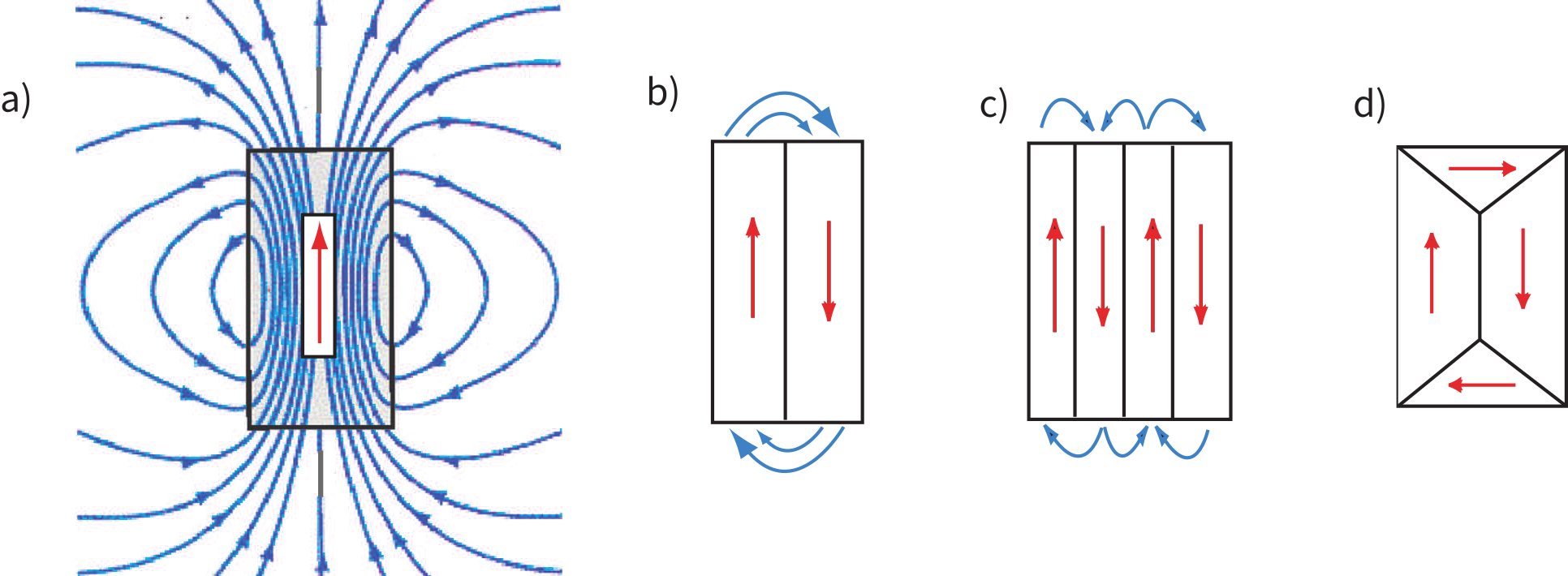
Figure 4.6:A variety of domain structures of a given particle. a) Uniformly magnetized (single domain). [Adapted from Tipler (1999).] b) Two domains. c) Four domains in a lamellar pattern. d) Essentially two domains with two closure domains.
As you might already suspect, domain walls are not “free”, energetically speaking. If, as in Figure 4.7a, the spins simply switch from one orientation to the other abruptly, the exchange energy cost would be very high. One way to get around this is to spread the change over several hundred atoms, as sketched in Figure 4.7b. The wall width is wider and the exchange energy price is much less. However, there are now spins in unfavorable directions from a magnetocrystalline point of view (they are in “hard” directions). Exchange energy therefore favors wider domain walls while magnetocrystalline anisotropy favors thin walls. With some work (see e.g., Dunlop & Özdemir (1997), pp. 117–118), it is possible to come up with the following analytical expressions for wall width () and wall energy density ():
where is the exchange constant (see Section 4.1.1) and is the magnetic anisotropy constant (e.g., or ). Note that is the energy density per unit wall area, not per volume. Plugging in values for magnetite given previously we get = 90 nm and = 3×10 Jm.
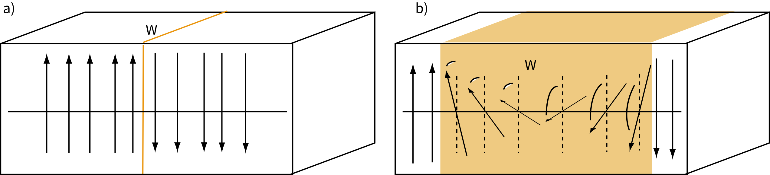
Figure 4.7:Examples of possible domain walls. a) There is a 180° switch from one atom to the next. The domain wall is very thin, but the exchange price is very high. b) There is a more gradual switch from one direction to the other [note: each arrow represents several 10’s of unit cells]. The exchange energy price is lower, but there are more spins in unfavorable directions from a magnetocrystalline point of view.
In Figure 4.8 we plot the self energy (Equation 4.13) and the wall energy ( from Equation 4.15) for spheres of magnetite. We see that the wall energy in particles with diameters of some 50 nm is less than the self energy, yet the width of the walls is about twice as wide as that. So the smallest wall is really more like the vortex state and it is only for particles larger than a few tenths of a micron that true domains separated by discrete walls can form. Interestingly, this is precisely what is predicted from micromagnetic modelling (e.g., Figure 4.5).
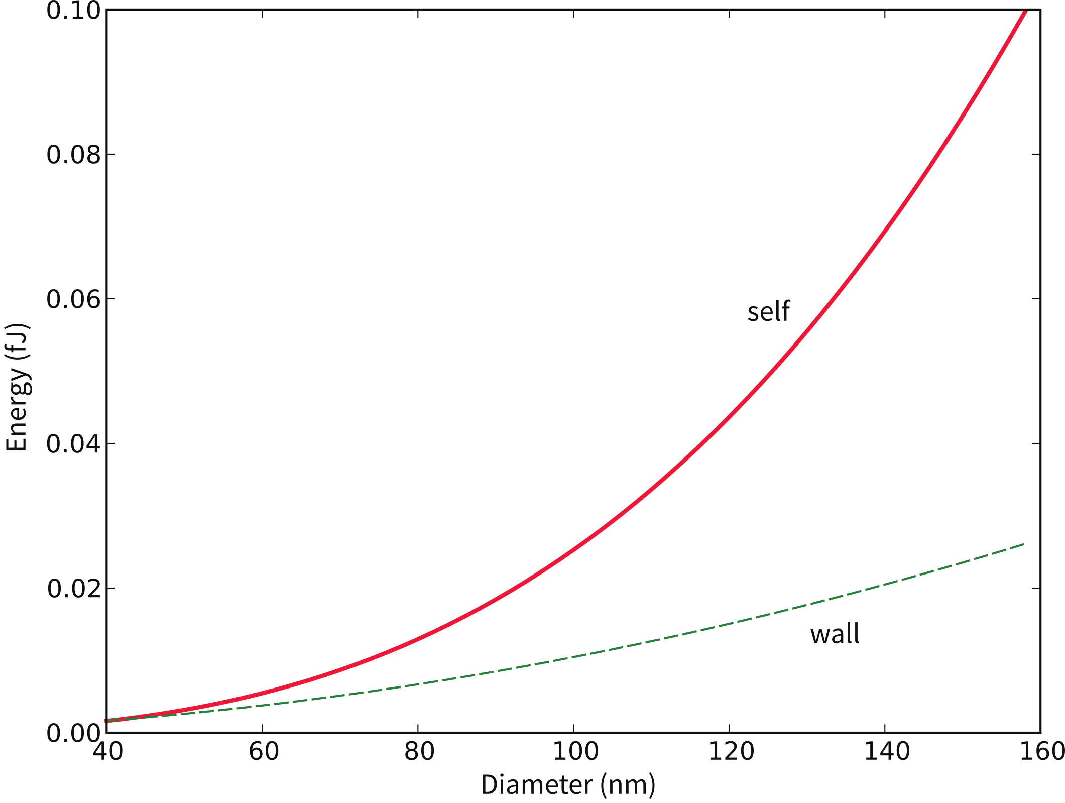
Figure 4.8:Comparison of “self” energy versus the energy of the domain wall in magnetite spheres as a function of particle size.
How can we test the theoretical predictions of domain theory? Do domains really exist? Are they the size and shape we expect? Are there as many as we would expect? In order to address these questions we require a way of imaging magnetic domains. Bitter (1931) devised a way for doing just that. Magnetic domain walls are regions with large stray fields (as opposed to domains in which the spins are usually parallel to the sides of the crystals to minimize stray fields). In the Bitter technique magnetic colloid material is drawn to the regions of high field gradients on highly polished sections allowing the domain walls to be observed (see Figure 4.9a).
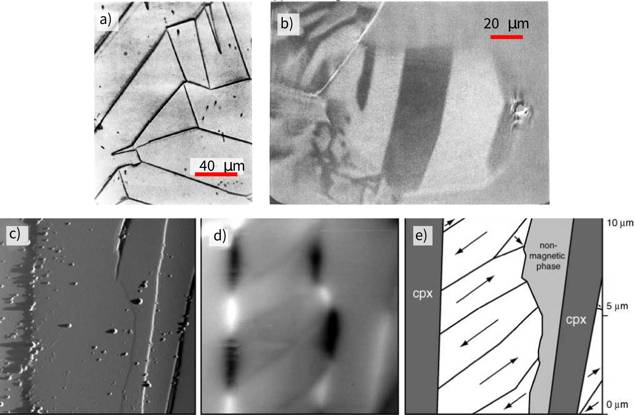
Figure 4.9:a) Bitter patterns from an oriented polished section of magnetite. [Figure from Özdemir et al. (1995).] b) Domains revealed by longitudinal magneto-optical Kerr effect. [Image from Heider & Hoffmann (1992).] c–e) Magnetic force microscopy technique. [Images from Feinberg et al. (2005).] c) Image of topography of surface of a magnetite inclusion in a non-magnetic matrix. d) Magnetic image from MFM technique. e) Interpretation of magnetizations of magnetic domains.
There are by now other ways of imaging magnetic domains. We will not review them all here, but will just highlight the ways that are more commonly used in rock and paleomagnetism. The magneto-optical Kerr effect or MOKE uses the interaction between polarized light and the surface magnetic field of the target. The light interacts with the magnetic field of the sample which causes a small change in the light’s polarization and ellipticity. The changes are detected by reflecting the light into nearly-crossed polarizers. The longitudinal Kerr effect can show the alignment of magnetic moments in the surface plane of the sample. Domains with different magnetization directions show up as lighter or darker regions in the MOKE image (see Figure 4.9b.)
Another common method for imaging magnetic domains employs a technique known as magnetic force microscopy. Magnetic force microscopy (MFM) uses a scanning probe microscope that maps out the vertical component of the magnetic fields produced by a highly polished section. The measurements are made with a cantilevered magnetic tip that responds to the magnetic field of the sample. In practice, the measurements are made in two passes. The first establishes the topography of the sample (Figure 4.9c). Then in the second pass, the tip is raised slightly above the surface and by subtracting the “topographic only” signal the attraction of the magnetic surface can be mapped (Figure 4.9d). Figure 4.9e shows an interpretation of the magnetic directions of different magnetic domains.
4.3Thermal energy
We have gone some way toward answering the questions posed at the beginning of the chapter. We see now that anisotropy energy, with contributions from crystal structure, shape and stress, inhibits changes in the magnetic direction thereby offering a possible mechanism whereby a given magnetization could be preserved for posterity. We also asked the question of what allows the magnetization to come into equilibrium with the applied magnetic field in the first place; this question requires a little more work to answer. The key to this question is to find some mechanism which allows the moments to “jump over” magnetic anisotropy energy barriers. One such mechanism is thermal energy , which was given in Chapter 3 as:
We know from statistical mechanics that the probability of finding a grain with a given thermal energy sufficient to overcome some anisotropy energy and change from one easy axis to another is . Depending on the temperature, such grains may be quite rare, and we may have to wait some time for a particle to work itself up to jumping over the energy barrier.
Imagine a block of material containing a random assemblage of magnetic particles that are for simplicity uniformly magnetized and dominated by uniaxial anisotropy. Suppose that this block has some initial magnetization and is placed in an environment with no ambient magnetic field. Anisotropy energy will tend to keep each tiny magnetic moment in its original direction and the magnetization will not change over time. At some temperature, certain grains will have sufficient energy to overcome the anisotropy energy and flip their moments to the other easy axis. As a result, over time, the magnetic moments will become random. Therefore, the magnetization as a function of time in this simple scenario will decay to zero. The equation governing this decay is:
where is time and the relaxation time. Relaxation time is the time required for the remanence to decay to of . This equation is the essence of what is called Néel theory (see Néel (1955)).
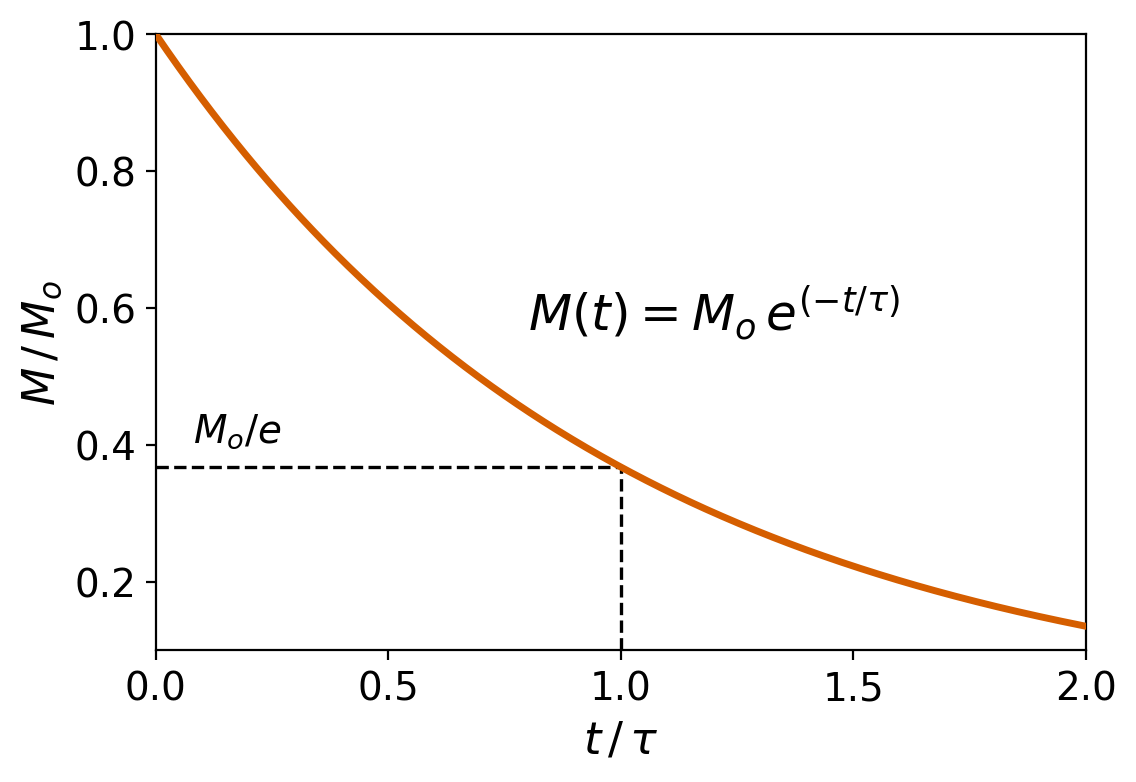
Figure 4.10:Magnetic relaxation in an assemblage of single domain ferromagnetic grains. The initial magnetization decays exponentially, falling to (~37%) of its original strength in time . For example, for grains with a relaxation time () of 100 s, 63% of the original magnetization is lost within 100 seconds.
The value of the relaxation time () depends on the competition between magnetic anisotropy energy and thermal energy. It is a measure of the probability that a grain will have sufficient thermal energy to overcome the anisotropy energy and switch its moment. Therefore in zero external field:
where is a frequency factor with a value of something like 1010 s. The anisotropy energy is given by the dominant anisotropy parameter (either , or ) times the grain volume .
Thus, the relaxation time is proportional to anisotropy constant and volume, and is inversely related to temperature. In Chapter 7, we will see how these relationships are central to rock’s acquiring (and losing) magnetization. Relaxation time varies rapidly with small changes in and . To see how this works, we can take for slightly elongate cuboids of magnetite (length to width ratio of 1.3 to 1) and evaluate relaxation time as a function of particle width (see Figure 4.11). There is a sharp transition between grains with virtually no stability ( is on the order of seconds) and grains with stabilities of billions of years.
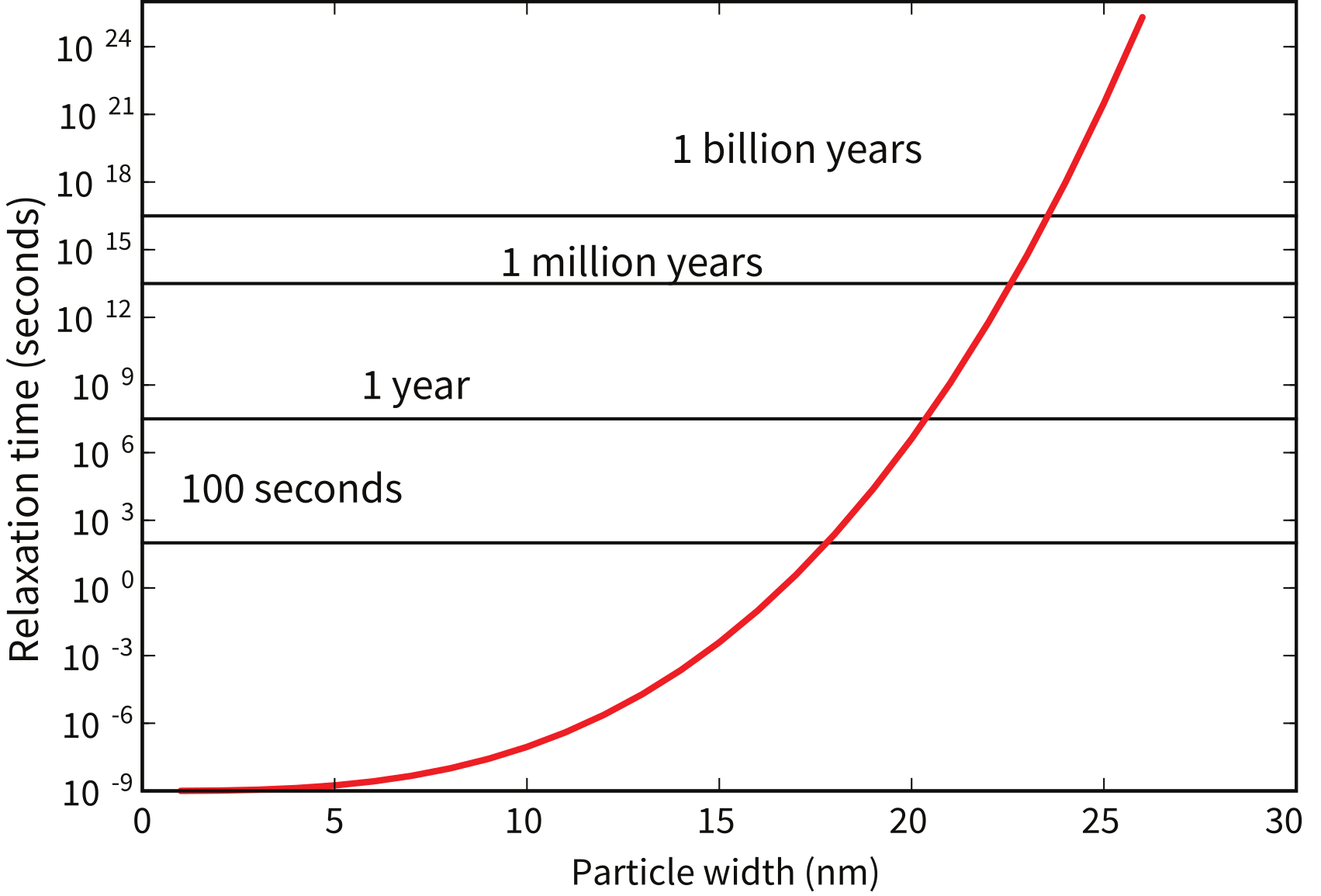
Figure 4.11:Relaxation time in magnetite ellipsoids as a function of grain width in nanometers (all length to width ratios of 1.3:1.)
Grains with seconds have sufficient thermal energy to overcome the anisotropy energy frequently and are unstable on a laboratory time scale. In zero field, these grain moments will tend to rapidly become random, and in an applied field, also tend to align rapidly with the field. The net magnetization is related to the field by a Langevin function (see Chapter 3). Therefore, this behavior is quite similar to paramagnetism, hence these grains are called superparamagnetic (SP). Such grains can be distinguished from paramagnets, however, because the field required to saturate the moments is typically much less than a tesla, whereas that for paramagnets can exceed hundreds of tesla.
4.4Putting it all together
We are now in a position to pull together all the threads we have considered in this chapter and make a plot of what sort of magnetic particles behave as superparamagnets, which should be single domain and which should be multidomain according to our simple theories. We can estimate the superparamagnetic to single domain threshold for magnetite as a function of particle shape by finding the length (2a) that gives a relaxation time of 100 seconds as a function of width-to-length ratio () for parallelepipeds of magnetite (heavy blue line in Figure 4.12). To do this, we follow the logic of Evans & McElhinny (1969) and Butler & Banerjee (1975). In this Evans diagram, we estimated relaxation time using Equation 4.18, plugging in values of as either the magnetocrystalline effective anisotropy constant () or the shape anisotropy constant (), whichever was less. We also show the curve at which relaxation time is equal to 1 Gyr, reinforcing the point that very small changes in crystal size and shape make profound differences in relaxation time. The figure also predicts the boundary between the single domain field and the two domain field, when the energy of a domain wall is less than the self energy of a particle that is uniformly magnetized. This can be done by evaluating wall energy with Equation 4.15 for a wall along the length of a parallelepiped and area () as compared to the self energy () for a given length and width-to-length ratio. When the wall energy is less than the self energy, we are in the two domain field.
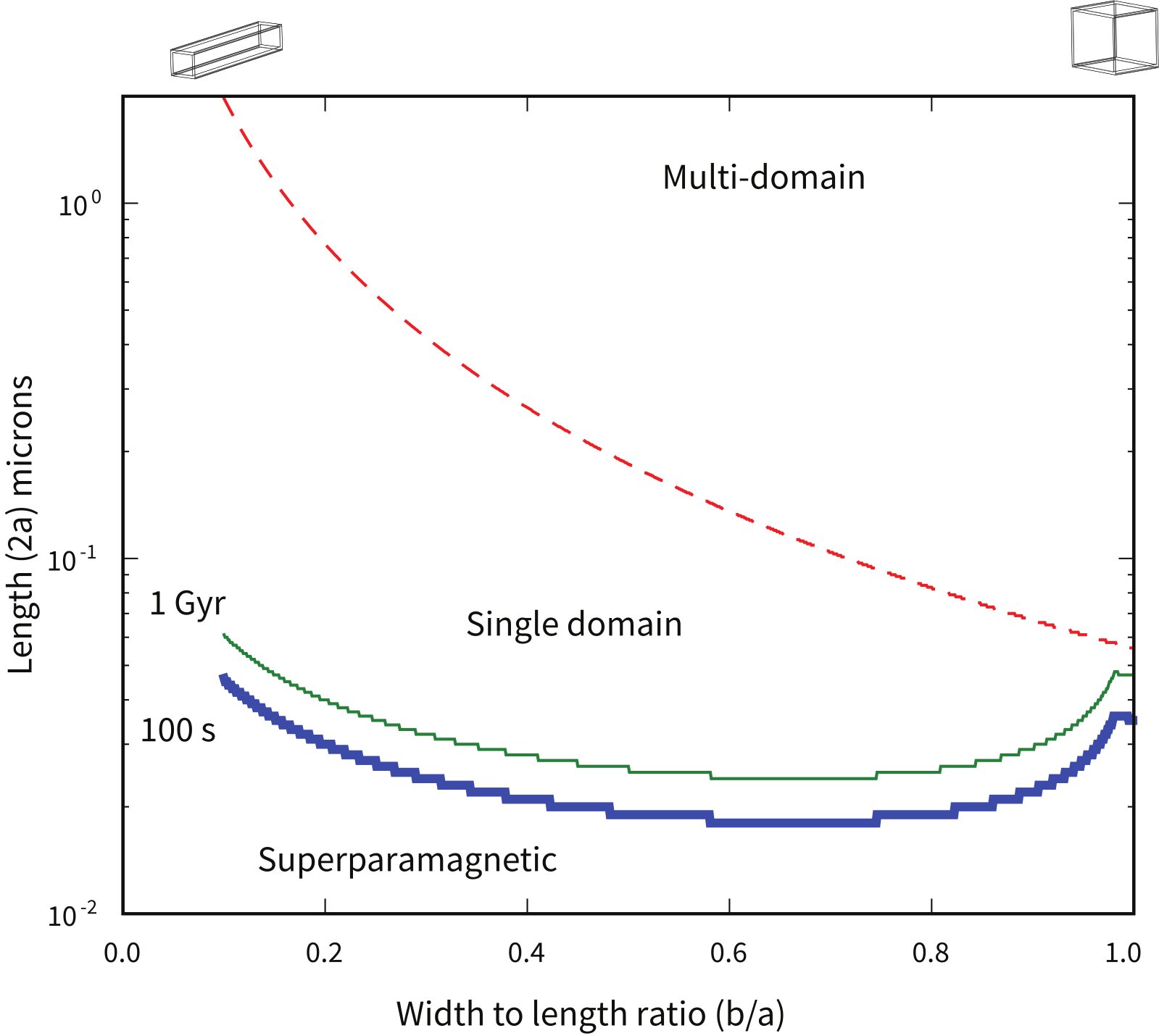
Figure 4.12:Expected domain states for various sizes and shapes of parallelepipeds of magnetite at room temperature. The parameters and are as in Figure 4.4e. Heavy blue (thin green) line is the superparamagnetic threshold assuming a relaxation time of 100s (1 Gyr). Dashed red line marks the SD/MD threshold size. Calculations done using assumptions and parameters described in the text.
Figure 4.12 suggests that there is virtually no SD stability field for equant magnetite; particles are either SP or MD (multidomain). As the width-to-length ratio decreases (the particle gets longer), the stability field for SD magnetite expands. Of course micromagnetic modelling shows that there are several transitional states between uniform magnetization (SD) and MD, i.e. the flower and vortex remanent states (see Fabian et al. (1996)), but Figure 4.12 has enormous predictive power and the version of Butler & Banerjee (1975) (which is slightly different in detail) continues to be used extensively. It is worth pointing out however, that the size at which domain walls appear in magnetite is poorly constrained because it depends critically on the exact shape of the particle, its state of stress and even its history of exposure to past fields. Estimates in the literature range from as small as 20 nm to much larger (up to 100 nm) depending on how the estimates are made. Nonetheless, it is probably true that truly single domain magnetite is quite rare in nature, yet more complicated states are difficult to treat theoretically. Therefore most paleomagnetic studies rely on predictions made for single domain particles.
Supplemental Reading: Dunlop & Özdemir (1997), Chapters 2.8 and 5.
4.5Problems
Problem 1
Assume that the magnetization of magnetite is about 4.8 × 10 Am. Using values for other parameters from the text, write a Python program to calculate the following:
a) Self energy (or magnetostatic energy) for a sphere 1, 10 and 100 m in diameter. [Hint: see Equation 4.13 for the ‘self’ energy density. Also, remember the difference between energy and energy density!]
b) Magnetostatic (shape) anisotropy energy for an ellipsoid whose principal semi-axis is 1 m and whose major and minor semi-axes are each 0.25 m. You may use the “nearly spherical” approximation in the text.
c) The critical radius of a sphere at which wall energy equals self energy.
Problem 2
Calculate grain diameter for magnetite spheres with s of 10, 10, 10, 10, 10, 10, 10 seconds. Use values for Boltzmann’s constant, (the frequency factor) and at room temperature (300K).
Problem 3 [From Jeff Gee]
a) Consider a highly elongate rod (needle-shaped grain) of magnetite. Explain why the demagnetizing factor along the long axis of the rod is about zero while that across the long axis is about one half.
b) The file Chapter_4/prolate.txt gives the values of demagnetizing factors for a prolate ellipsoid (with axes a > b = c). For an elongate rod of magnetite with range of aspect ratios (AR = c:b) provided in the table, plot the magnetostatic self energy density in the absence of an external field. Use this plot to estimate the aspect ratio at which shape anisotropy will be equal to that of magnetocrystalline anisotropy (use a value of at room temperature (300K) of −1.43 × 10 J/m).
c) What is the maximum microscopic coercivity () for such an elongate grain of magnetite (assume an infinitely long grain)? Coercivities are more commonly reported in units of T so provide this corresponding value as well.
- Williams, W., & Dunlop, D. J. (1995). Simulation of magnetic hysteresis in pseudo-single-domain grains of magnetite. Journal of Geophysical Research: Solid Earth, 100(B3), 3859–3871. 10.1029/94JB02878
- Syono, Y., & Ishikawa, Y. (1963). Magnetocrystalline anisotropy of xFe₂TiO₄·(1-x)Fe₃O₄. Journal of the Physical Society of Japan, 18, 1230–1231. 10.1143/JPSJ.18.1230
- Fletcher, E. J., & O’Reilly, W. (1974). Contribution of Fe2+ ions to the magnetocrystalline anisotropy constant K₁ of Fe₃₋ₓTiₓO₄. Journal of Physics C: Solid State Physics, 7(1), 171–178. 10.1088/0022-3719/7/1/024
- Swanson-Hysell, N. L., Avery, M. S., Zhang, Y., Hodgin, E. B., Sherwood, R. J., Apen, F. E., Boerboom, T. J., Keller, C. B., & Cottle, J. M. (2021). The paleogeography of Laurentia in its early years: new constraints from the Paleoproterozoic East Central Minnesota batholith. Tectonics, 40(9), e2021TC006751. 10.1029/2021TC006751
- Dunlop, D. J., & Özdemir, Ö. (1997). Rock Magnetism: Fundamentals and Frontiers. Cambridge University Press. 10.1017/CBO9780511612794
- Martı́n-Hernández, Fa., & Guerrero-Suárez, S. (2012). Magnetic anisotropy of hematite natural crystals: high field experiments. International Journal of Earth Sciences, 101(3), 637–647. 10.1007/s00531-011-0665-z
- Moskowitz, B. M. (1993). High-temperature magnetostriction of magnetite and titanomagnetites. Journal of Geophysical Research: Solid Earth, 98(B1), 359–371. 10.1029/92JB01846
- O’Reilly, W. (1984). Rock and Mineral Magnetism. Blackie. 10.1007/978-1-4684-8468-7
- Stacey, F. D., & Banerjee, S. K. (1974). The Physical Principles of Rock Magnetism. Elsevier.
- Nagata, T. (1961). Rock Magnetism (2nd ed.). Maruzen.
- Nagy, L., Williams, W., Muxworthy, A. R., Fabian, K., Almeida, T. P., Ó Conbhuí, P., & Shcherbakov, V. P. (2017). Stability of equidimensional pseudo-single-domain magnetite over billion-year timescales. Proceedings of the National Academy of Sciences, 114(39), 10356–10360. 10.1073/pnas.1708344114
- Williams, W., Moreno, R., Muxworthy, A. R., Paterson, G. A., Nagy, L., Tauxe, L., Bellon, U. D., Cowan, A. A., & Ferreira, I. (2024). Vortex magnetic domain state behavior in the Day plot. Geochemistry, Geophysics, Geosystems, 25(8), e2024GC011462. 10.1029/2024GC011462
- Ó Conbhuí, P., Williams, W., Fabian, K., Ridley, P., Nagy, L., & Muxworthy, A. R. (2018). MERRILL: Micromagnetic Earth Related Robust Interpreted Language Laboratory. Geochemistry, Geophysics, Geosystems, 19(4), 1080–1106. 10.1002/2017GC007279
- Tipler, P. A. (1999). Physics for Scientists and Engineers (4th ed.). W. H. Freeman.
- Bitter, F. (1931). On inhomogeneities in the magnetization of ferromagnetic materials. Physical Review, 38(10), 1903–1905. 10.1103/PhysRev.38.1903