D.1The 15 measurement protocol
The Jelı́nek (1978) 15 measurement scheme is illustrated in Figure D.1. This is the procedure recommended in the manual distributed with the popular Kappabridge susceptibility instruments. In the 15 measurement case shown in Figure D.1, the design matrix is:
and
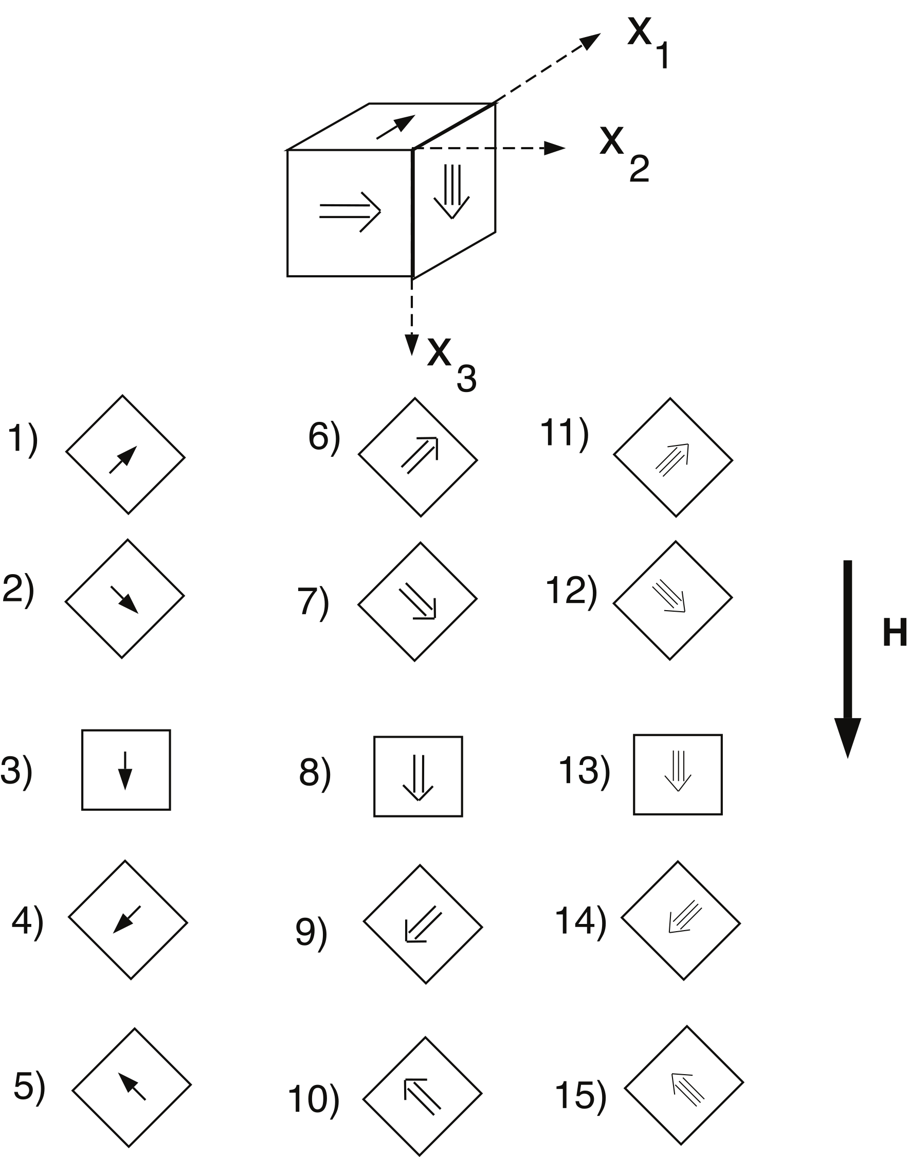
Figure D.1:The 15 position scheme of Jelı́nek (1978) for measuring the AMS of a sample. [Figure from Tauxe (1998).]
D.2The spinning protocol
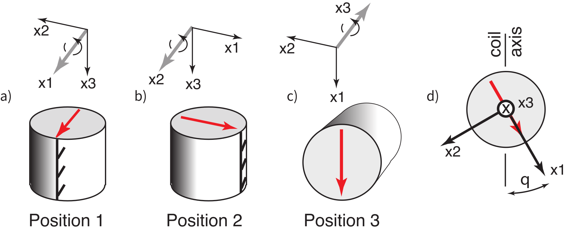
Figure D.2:Specimen orientations for the three spins used with spinning magnetic susceptibility meters. The heavy gray arrows show the axes of rotation; one oriented toward the user for Position 1 (a) and 2 (b) away from the user for Position 3 (c). The orientation of the specimen coordinate system in space is specified by the azimuth and plunge of either the arrow along the core length (+x axis, black) or the +x axis (red arrow on core top). d) orientation of applied field (coil axis) relative to specimen coordinates in Position 3. [Figure from Gee et al. (2008).]
More recent models of the Kappabridge magnetic susceptibility instruments (e.g., KLY-3S and KLY-4S; see e.g., Pokorný et al. (2004)) measure anisotropy by spinning the specimen around three axes (Figure D.2). For complete measurement and analysis details, see Gee et al. (2008). Here we just give the bare bones explanation.
The specimen is lowered into the measurement region and the susceptibility meter is set to zero. The deviatoric susceptibility is then measured in 64 positions per revolution for multiple (often eight) revolutions (see Figure D.3a). These data must be corrected for instrumental drift (red line in the figure), adjusted to have zero mean and stacked (Figure D.3b). The data can be fit with a best fit theoretical curve (red line in the figure). The theoretical curve can be derived from the complicated design matrix (see Gee et al. (2008) for details). As one example, the measurement recorded at an angle (as shown in Figure D.2d) while spinning in Position 1 (Figure D.2a) is given by:
The best fit values for for the entire sequence of data gives the 2D Model for the set of data (see Figure D.3b). There are three such models for the measurement protocol, each yielding estimates of two of the three on-axis values (). These measurements are all adjusted to zero mean susceptibility so one more measurement is required to determine the bulk susceptibility (the absolute susceptibility measured in the position shown in Figure D.2c or in Position 3). The three 2D models plus the bulk measurement are combined as shown in Figure D.3d whereby the position in the 2D model for Position 3 is adjusted to the bulk measurement, and the best-fit 3D model is found that minimizes cross over errors for pairs of . Once the best fit values for are found and standard deviation, the data can be treated as described in Chapter 13.
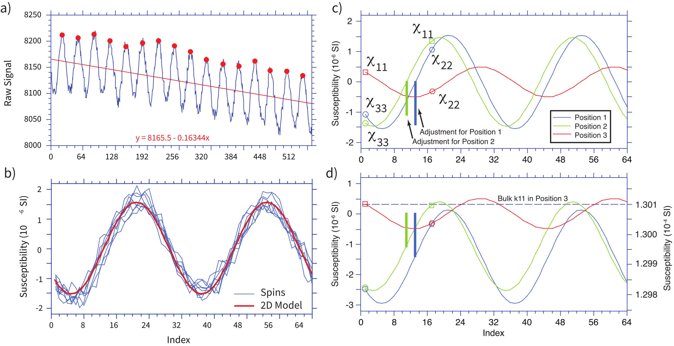
Figure D.3:Processing steps for data spin protocol. a) From a single spin with eight revolutions. Raw data with peaks (red dots) identified by peak-finding algorithm and best fit linear trend. Data are detrended using peaks. b) Data from detrended individual revolutions and best fit 2-D model. c) Original (zero-mean) deviatoric susceptibility data from three spins. The best fit 2-D model for each spin provides an estimate of two elements of the deviatoric susceptibility tensor (square, ; hexagon, ; circle, ). Thick bars indicate the calculated offsets for Positions 1 and 2. d) Crossover adjustment for data from three positions. Original (zero-mean) deviatoric susceptibility data from three positions are scaled to absolute values (right-hand scale) using a bulk measurement in spin Position 3, and adjusted to minimize cross over error. [Figure modified from Gee et al. (2008).]
D.3Correction of inclination error with AARM
The magnitude of ARM is here denoted . The particle anisotropy is denoted and is given by:
where and are the magnitudes of the ARM acquired parallel to and perpendicular to the detrital particle long axis respectively. The normalized eigenvalues of the ARM tensor () are defined as:
Stephenson et al. (1986) defined an orientation distribution function for the preferred alignment of particle long axes whose eigenvalues are given by where as usual. Jackson et al. (1991) collect together the two sources of anisotropy (alignment of particle long axes and individual particle anisotropies) as:
Assuming that the DRM anisotropy is identical to the orientation distribution function of particle long axes we can combine and rearrange Equation 13.23 and Equation D.7 to get the relationship between the flattening factor and the ARM anisotropy:
From the foregoing, measuring the AARM tensor yields the values for , but determining values for are more problematic. Vaughn et al. (2005) describe a technique whereby magnetic particles are separated from the matrix, then allowed to dry in an epoxy matrix in the presence of a magnetic field sufficient to fully align the long axes of the magnetic particles (say 50 mT). The AARM parallel to and perpendicular to the axis of alignment therefore gives by Equation D.5.
- Jelı́nek, V. (1978). Statistical processing of anisotropy of magnetic susceptibility measured on groups of specimens. Studia Geophysica et Geodaetica, 22(1), 50–62. 10.1007/BF01613632
- Tauxe, L. (1998). Paleomagnetic Principles and Practice. Kluwer Academic Publishers.
- Gee, J. S., Tauxe, L., & Constable, C. (2008). AMSSpin: A LabVIEW program for measuring the anisotropy of magnetic susceptibility with the Kappabridge KLY-4S. Geochemistry, Geophysics, Geosystems, 9(8), Q08Y02. 10.1029/2008GC001976
- Pokorný, J., Suza, P., & Hrouda, F. (2004). Anisotropy of magnetic susceptibility of rocks measured in variable weak magnetic fields using the KLY-4S Kappabridge. In F. Martín-Hernández, C. M. Lüneburg, C. Aubourg, & M. Jackson (Eds.), Magnetic Fabric: Methods and Applications (Vol. 238, pp. 69–76). Geological Society, London, Special Publications. 10.1144/GSL.SP.2004.238.01.05
- Stephenson, A., Sadikun, S., & Potter, D. K. (1986). A theoretical and experimental comparison of the anisotropies of magnetic susceptibility and remanence in rocks and minerals. Geophysical Journal of the Royal Astronomical Society, 84(1), 185–200. 10.1111/j.1365-246X.1986.tb04351.x
- Jackson, M. J., Banerjee, S. K., Marvin, J. A., Lu, R., & Gruber, W. (1991). Detrital remanence, inclination errors and anhysteretic remanence anisotropy: quantitative model and experimental results. Geophysical Journal International, 104(1), 95–103. 10.1111/j.1365-246X.1991.tb02496.x
- Vaughn, J., Kodama, K. P., & Smith, D. P. (2005). Correction of inclination shallowing and its tectonic implications: The Cretaceous Perforada Formation, Baja California. Earth and Planetary Science Letters, 232(1–2), 71–82. 10.1016/j.epsl.2004.12.021