
Hysteresis Processing walkthrough notebook#
This notebook provides a step-by-step walk through of the processing of hysteresis loops. Each processing step is illustrated and described. This walk through can enable more granular data processing and illustrates the decision tree that is automatically implemented in the hysteresis_processing.ipynb.
Install and import packages#
import pmagpy.rockmag as rmag
import pmagpy.ipmag as ipmag
import pmagpy.contribution_builder as cb

from bokeh.plotting import figure, show
from bokeh.io import output_notebook
output_notebook(hide_banner=True)
Import local data in MagIC format#
In this demonstration we will be using local data.
The data is from the following publication:
Swanson-Hysell, N. L., Avery, M. S., Zhang, Y., Hodgin, E. B., Sherwood, R. J., Apen, F. E., et al. (2021). The paleogeography of Laurentia in its early years: New constraints from the Paleoproterozoic East-Central Minnesota Batholith. Tectonics, 40, e2021TC006751. https://doi.org/10.1029/2021TC006751
# set the dir_path to the directory where the measurements.txt file is located
dir_path = '../example_data/ECMB'

# set the name of the MagIC file
ipmag.unpack_magic('magic_contribution_20213.txt',
                     dir_path = dir_path,
                     input_dir_path = dir_path,
                     print_progress=False)

# create a contribution object from the tables in the directory
contribution = cb.Contribution(dir_path)
measurements = contribution.tables['measurements'].df
1  records written to file  /Users/yimingzhang/Github/RockmagPy-notebooks/example_data/ECMB/contribution.txt
1  records written to file  /Users/yimingzhang/Github/RockmagPy-notebooks/example_data/ECMB/locations.txt
90  records written to file  /Users/yimingzhang/Github/RockmagPy-notebooks/example_data/ECMB/sites.txt
312  records written to file  /Users/yimingzhang/Github/RockmagPy-notebooks/example_data/ECMB/samples.txt
1574  records written to file  /Users/yimingzhang/Github/RockmagPy-notebooks/example_data/ECMB/specimens.txt
17428  records written to file  /Users/yimingzhang/Github/RockmagPy-notebooks/example_data/ECMB/measurements.txt
-I- Using online data model
-I- Getting method codes from earthref.org
-I- Importing controlled vocabularies from https://earthref.org
Get hysteresis data from the \(measurements\) variable#
The method codes relevant to hysteresis loops are:
LP-HYSfor regular hysteresis loopsLP-HYS-Ofor hysteresis loops as a function of orientationLP-HYS-Tfor hysteresis loops as a function of temperature
Inspect the original measurement level data#
Below we investigate all the available specimens that have hysteresis data in the database for this contribution.
We extract the experimental data for an individual specimen.
measurements = measurements[measurements['method_codes'] == 'LP-HYS']
measurements.specimen.unique()
array(['NED1-5c', 'NED18-2c', 'NED2-8c', 'NED4-1c', 'NED6-6c'],
      dtype=object)
# filter and isolate specimen specific hysteresis loop data by specimen name
NED1_5c_hyst = measurements[measurements['specimen'] == 'NED1-5c'].reset_index(drop=True)
NED18_2c_hyst = measurements[measurements['specimen'] == 'NED18-2c'].reset_index(drop=True)
NED2_8c_hyst = measurements[measurements['specimen'] == 'NED2-8c'].reset_index(drop=True)
NED4_1c_hyst = measurements[measurements['specimen'] == 'NED4-1c'].reset_index(drop=True)
NED6_6c_hyst = measurements[measurements['specimen'] == 'NED6-6c'].reset_index(drop=True)
Let’s take a look at the columns relevant to hysteresis data processing
magn_massis mass normalized magnetization (in Am^2/kg)meas_field_dcis the applied DC field (in T)
NED18_2c_hyst[['magn_mass', 'meas_field_dc']]
| magn_mass | meas_field_dc | |
|---|---|---|
| 0 | 0.2827 | 1.0000 |
| 1 | 0.2825 | 0.9989 |
| 2 | 0.2820 | 0.9960 |
| 3 | 0.2813 | 0.9919 |
| 4 | 0.2806 | 0.9873 |
| ... | ... | ... |
| 797 | 0.2760 | 0.9728 |
| 798 | 0.2768 | 0.9777 |
| 799 | 0.2777 | 0.9828 |
| 800 | 0.2786 | 0.9878 |
| 801 | 0.2805 | 1.0000 |
802 rows × 2 columns
Visualize the raw data with plot_hysteresis_loop#
The function returns a Bokeh plot object which can be further customized before displaying
NED18_2c_plot = rmag.plot_hysteresis_loop(NED18_2c_hyst['meas_field_dc'], NED18_2c_hyst['magn_mass'],
                                          'NED18-2c', line_color='orange', line_width=1, label='NED18-2c')
show(NED18_2c_plot)
Loop processing#
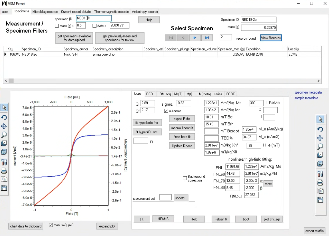
rockmagpy calculates the hysteresis loop parameters as available in the IRMDB software. Summary parameters can then be exported into the MagIC specimen data table.
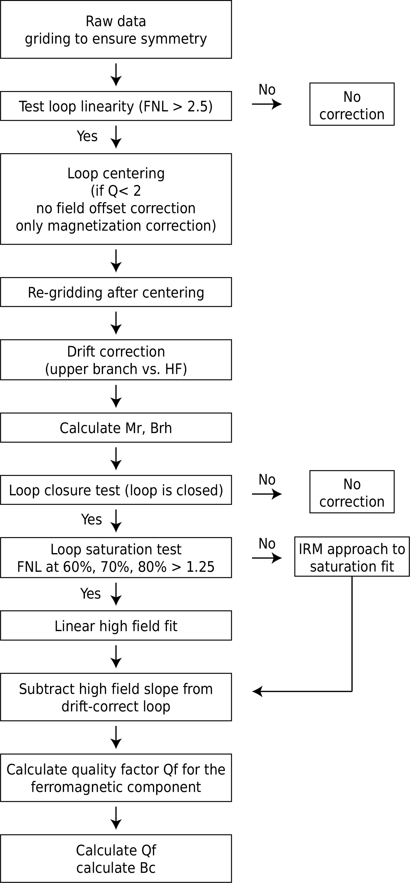
The processing functions generally follow the workflow presented in Paterson et al., 2018 which is modified upon the workflow presented in Jackson and Solheid, 2010. This flowchart shows the decision tree for data processing.
Interpolate the raw data and re-grid them into an upper and a lower branch with exactly the same and symmetric field steps#
The applied DC field values through the upper and lower branches during experiments are usually not exactly symmetric about the origin. We need to correct for the slight mismatching between the field steps by splitting the loop into an upper branch and a lower branch, interpolating the branches and unifying their field axis to be the same and be symmetric about 0.
The function
rmag.grid_hysteresis_loopaccomplishes this task.
NED18_2c_hyst_grid_field, NED18_2c_hyst_grid_magnetization = rmag.grid_hysteresis_loop(NED18_2c_hyst['meas_field_dc'],
                                                                                       NED18_2c_hyst['magn_mass'])

NED18_2c_plot_grid = rmag.plot_hysteresis_loop(NED18_2c_hyst_grid_field, NED18_2c_hyst_grid_magnetization, specimen_name='NED18-2c',
                                               p=NED18_2c_plot, line_color='orange', label='NED18-2c gridded', legend_location='top_left')
show(NED18_2c_plot_grid)
Perform linearity test on the whole loop#
If the whole loop is linear, the sample is dominated by paramagnetic or diamagnetic materials
If the whole loop is not linear, we should move on to further processing
The
FNLtest statistic is based on the ANOVA testThe resultant stats from function
hyst_linearity_testhas an attribute ‘loop is linear’ which is a boolean value that signals whether the loop is linear or not
loop_linearity = rmag.hyst_linearity_test(NED18_2c_hyst_grid_field, NED18_2c_hyst_grid_magnetization)
loop_linearity
{'SST': 31.403041872524103,
 'SSR': 29.9952402479435,
 'SSD': 1.4078016245806735,
 'R_squared': 0.9551698962700697,
 'SSPE': 0.00011833105860016647,
 'SSLF': 1.4076832935220733,
 'MSPE': 2.943558671645932e-07,
 'MSLF': 0.0035192082338051833,
 'MSR': 29.9952402479435,
 'MSD': 0.0017553636216716627,
 'FL': 17087.764539280197,
 'FNL': 11955.62455643994,
 'slope': 0.33403964536277,
 'intercept': 3.210002097500637e-05,
 'loop_is_linear': False}
Loop centering#
In the example case, the loop is not linear, so we need to isolate the ferromagnetic component from the paramagnetic component.
We need to center the loop to remove any offset in the field and moment axes that could be present in the data.
centering_results = rmag.hyst_loop_centering(NED18_2c_hyst_grid_field, NED18_2c_hyst_grid_magnetization)
NED18_2c_hyst_centered_H, NED18_2c_hyst_centered_M = centering_results['centered_H'], centering_results['centered_M']
NED18_2c_plot_centered = rmag.plot_hysteresis_loop(NED18_2c_hyst_centered_H, NED18_2c_hyst_centered_M, specimen_name='NED18-2c', p=NED18_2c_plot_grid, line_color='red', label='NED18-2c offset corrected', legend_location='top_left')
show(NED18_2c_plot_centered)
Quality factor Q#
Once the loop has been centered, the quality factor Q can be calculated. ‘Q’ is calculated as the decimal log of the signal/noise ratio, calculated from the mean square mismatch between symmetrically equivalent moments. A higher value indicates better quality data. Note this value deviates from that currently calculated in the IRM VSM Ferret as that value is estimated from the FNL statistic.
High Q values (e.g., 2 or greater) indicate that deviations from inversion symmetry due to all possible sources (noise, drift, and inherent asymmetry) are small. Conversely, low values indicate that at least one of these is significant.
centering_results['Q']
2.410906494319133
Loop drift correction#
Sometimes spurious changes occur in measured signal strength on time scales comparable to that of the loop measurement. It is typically manifested by failure of loops to close, by lack of even symmetry in Mrh, and/or by failure of Mrh to decrease to zero in large (positive or negative) fields.
In many cases this is not strictly necessary as the drift signal is small, but nonetheless an approach is to by default look at the smoothed Me curve and determine whether a high field drift correction or upper branch drift correction is needed.
If you zoom in on the ~1T region of the loop above, you will find that there is a slight difference between the beginning and end points
In this case, we first correct the drift by subtracting a smoothed Me curve either at the high field region or the entire upper branch of the loop. This necessarily causes a shift in the upper branch that will cause additional asymmetry in the corrected loop.
NED18_2c_hyst_drift_corr_magnetization = rmag.drift_correction_Me(NED18_2c_hyst_centered_H, NED18_2c_hyst_centered_M)
NED18_2c_plot_drift_corr = rmag.plot_hysteresis_loop(NED18_2c_hyst_centered_H, NED18_2c_hyst_drift_corr_magnetization, specimen_name='NED18-2c', p=NED18_2c_plot_centered, line_color='blue', label='NED18-2c drift corrected', legend_location='top_left')
show(NED18_2c_plot_drift_corr)
calculate the Mr (remanent magnetization) Mrh (remanence component), Mih (induced component), Me (error), Brh (field corresponding to 1/2 Mr)#
The function
calc_Mr_Mrh_Mih_Brhcalculates these values and curves.Below we print out the Mr value and Brh value.
H, Mr, Mrh, Mih, Me, Brh = rmag.calc_Mr_Mrh_Mih_Brh(NED18_2c_hyst_centered_H, NED18_2c_hyst_drift_corr_magnetization)
print('Mr: ', Mr, 'Brh: ', Brh)
Mr: 0.01377229051354287 Brh: 0.03638378969652703
NED18_2c_plot_drift_corr.line(H, Mrh, line_color='green', legend_label='Mrh', line_width=1)
NED18_2c_plot_drift_corr.line(H, Mih, line_color='purple', legend_label='Mih', line_width=1)
NED18_2c_plot_drift_corr.line(H, Me, line_color='brown', legend_label='Me', line_width=1)
show(NED18_2c_plot_drift_corr)
Test loop closure#
When there are significant high coercivity components in the sample such as hematite or goethite, the hysteresis branches will not be overlapping at the highest applied fields
In that case, hysteresis processing interpretation should stop as we are not able to estimate Ms. We will report the total FNL, FNL60, FNL70, and FNL80 values, and Bc value
If the loop is closed, we move on to the next step of testing loop saturation
use H, Mrh and function
loop_open_testto test the loop closure
loop_closure_test = rmag.loop_closure_test(H, Mrh)
loop_closure_test['loop_is_closed']
True
Test loop saturation (high-field linearity test)#
In the example case, the loop is closed, so we proceed to test the loop saturation. This test allows us to determine the appropriate approach for fitting the high-field portion of the loop and determining Ms.
The lack of saturation can cause a loop to deviate from linearity at high fields. Although such a deviation from linearity can be subtle to the eye, it can have a significant effect on estimates of Ms. As developed in Jackson and Solheid (2010), a linearity test is conducted through 60%, 70%, and 80% of the maximum field range. If the loop statistically deviates from being linear at the highest fields, it would be inappropriate to use a linear fit to the high-field data to correct for the paramagnetic or diamagnetic slope for an accurate estimate of the saturation magnetization (Ms). If the loop is consistent with being linear at high fields, we then use the fraction of the high-field slope above the value corresponding to the positive linearity test (FNL).
In the example case, the loop is not saturated at 60%, 70%, and 80% of the maximum field range. Therefore, an approach to saturation fit needs to be used for isolating the ferromagnetic loop and then calculating the Ms and the high field susceptibility values.
loop_saturation_test_result = rmag.hyst_loop_saturation_test(NED18_2c_hyst_centered_H, NED18_2c_hyst_drift_corr_magnetization)
loop_saturation_test_result
{'FNL60': 39.70133189858125,
 'FNL70': 7.648391270777258,
 'FNL80': 2.792041361014829,
 'saturation_cutoff': 0.92,
 'loop_is_saturated': False}
Fit high-field slope and get the intercept as Ms#
In this case, the loop is not saturated at high fields and we should use an approach to saturation fit to calculate the Ms value.
But to show the difference between a linear fit and a saturation fit, we will also perform a linear fit on the high-field data and use the slope to correct the loop.
We use function
linear_HF_fitto estimate the paramagnetic slope (and the Ms intercept in case where the loop is saturated).We then use the resultant slope to correct the loop using the
hyst_slope_correctionfunction
slope, Ms = rmag.linear_HF_fit(NED18_2c_hyst_centered_H, NED18_2c_hyst_drift_corr_magnetization, loop_saturation_test_result['saturation_cutoff'])

NED18_2c_hyst_linear_ferro_M = rmag.hyst_slope_correction(NED18_2c_hyst_centered_H, NED18_2c_hyst_drift_corr_magnetization, slope)

print('Ms based on linear fitting: ', Ms)
Ms based on linear fitting: 0.11340116494190672
NED18_2c_plot_linear_ferro = rmag.plot_hysteresis_loop(NED18_2c_hyst_centered_H, NED18_2c_hyst_linear_ferro_M,
                                                       specimen_name='NED18-2c', p=NED18_2c_plot_drift_corr,
                                                       line_color='dodgerblue', label='NED18-2c linear high-field corrected')
show(NED18_2c_plot_linear_ferro)
Perform approach-to-saturation fit and estimate a more appropriate Ms#
In this example case, a linear fit would underestimate the Ms value.
A more appropriate Ms value can be estimated using a higher-order approach-to-saturation fit.
By default, we will use the IRM’s function
IRM_nonlinear_fitwhere $\(M = \chi_{HF} * H + Ms + a_1 * H^{-1} + a_2 * H^{-2}\)$
NL_fit_result = rmag.hyst_HF_nonlinear_optimization(NED18_2c_hyst_centered_H, NED18_2c_hyst_drift_corr_magnetization,
                                                    HF_cutoff=0.6, fit_type='IRM')

NL_fit_result
{'chi_HF': 2.0297572016074752e-07,
 'Ms': 0.12094525420612434,
 'a_1': -7.690491115462892e-17,
 'a_2': -0.0016265101865796702,
 'Fnl_lin': 2.0859246311264474}
Now let’s use the approach-to-saturation fit result to correct the loop.
NED18_2c_hyst_NL_ferro_M = rmag.hyst_slope_correction(NED18_2c_hyst_centered_H, NED18_2c_hyst_drift_corr_magnetization,
                                                      NL_fit_result['chi_HF'])
Plot the ferromagnetic component together with the previous intermediate products#
You may click on the legend items to hide the curves
The preferred final ferromagnetic component is shown in pink
NED18_2c_plot_NL_ferro = rmag.plot_hysteresis_loop(NED18_2c_hyst_centered_H, NED18_2c_hyst_NL_ferro_M,
                                                   specimen_name='NED18-2c', p=NED18_2c_plot_drift_corr,
                                                   line_color='pink', label='NED18-2c non-linear high-field correction',
                                                   legend_location='bottom_right')
show(NED18_2c_plot_NL_ferro)
inspect the differences between applying a linear high field slope fit vs. an approach-to-saturation fit#
high_field_fit_inspection_plot = rmag.plot_hysteresis_loop(NED18_2c_hyst_centered_H, NED18_2c_hyst_NL_ferro_M,
                                                   specimen_name='NED18-2c',
                                                   line_color='pink', label='NED18-2c non-linear high-field correction',
                                                   legend_location='bottom_right')
high_field_fit_inspection_plot = rmag.plot_hysteresis_loop(NED18_2c_hyst_centered_H, NED18_2c_hyst_linear_ferro_M,
                                                       specimen_name='NED18-2c', p=high_field_fit_inspection_plot,
                                                       line_color='dodgerblue', label='NED18-2c linear high-field corrected')

show(high_field_fit_inspection_plot)
Calculate the quality factor of the ferromagnetic component loop#
M_sn_f, Qf = rmag.calc_Q(NED18_2c_hyst_centered_H, NED18_2c_hyst_NL_ferro_M)
print('Qf: ', Qf)
Qf: 3.4489914970093496
Calculate Bc#
This calculation is based on the ferromagnetic component loop.
There will be a difference if you use the loops before high-field slope correction.
The Bc value is calculated as the average of the lower and upper branch.
The value shown is in unit of Tesla.
Bc = rmag.calc_Bc(NED18_2c_hyst_centered_H, NED18_2c_hyst_NL_ferro_M)
print('Bc: ', Bc)
Bc: 0.010025527047654427
The process_hyst_loop function#
The process_hyst_loop function applies all of the above steps using the decision tree to process the data.
NED18_2c_hyst_process_result = rmag.process_hyst_loop(NED18_2c_hyst['meas_field_dc'].values, NED18_2c_hyst['magn_mass'].values, 'NED18-2c')
References#
Jackson, M., & Solheid, P. (2010). On the quantitative analysis and evaluation of magnetic hysteresis data. Geochemistry, Geophysics, Geosystems, 11(4), Q04Z15. https://doi.org/10.1029/2009GC002932
Paterson, G. A., Zhao, X., Jackson, M., & Heslop, D. (2018). Measuring, processing, and analyzing hysteresis data. Geochemistry, Geophysics, Geosystems, 19(7), 1925–1945. https://doi.org/10.1029/2018GC007620
Swanson-Hysell, N. L., Avery, M. S., Zhang, Y., Hodgin, E. B., Sherwood, R. J., Apen, F. E., et al. (2021). The paleogeography of Laurentia in its early years: New constraints from the Paleoproterozoic East-Central Minnesota Batholith. Tectonics, 40, e2021TC006751. https://doi.org/10.1029/2021TC006751