
Plot MPMS data (AC susceptibility)#
This notebook visualizes data from low-temperature AC susceptibility (\(\chi\)) experiments conducted on an MPMS instrument and exported to MagIC format.
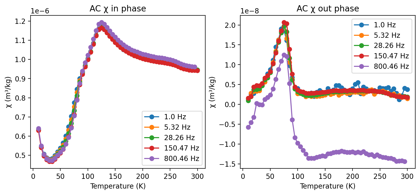
The response of magnetization to changes in an applied oscillating field is both dependent on time and temperature. Given that \(\chi\) can depend on frequency and temperature, experiments conducted on an MPMS will apply different frequency AC fields and make measurements as a function of temperature. The results of these experiments are visualized both in terms of the in-phase susceptibility (susc_chi_mass) and the out-of-phase susceptibility (susc_chi_qdr_mass)
Import scientific python libraries#
Run the cell below to import the functions needed for the notebook.
import pmagpy.rockmag as rmag
import pmagpy.contribution_builder as cb
import pmagpy.ipmag as ipmag
import pandas as pd
pd.set_option('display.max_columns', 500)
%config InlineBackend.figure_format = 'retina'

from bokeh.io import output_notebook, save
output_notebook(hide_banner=True)
Import data#
We take the approach described in the rockmag_data_unpack.ipynb notebook to bring MagIC data developed during an IRM Summer School project from a private workspace into the notebook as a Contribution.
#define these three parameters to match your data
magic_id = '20432'
share_key = 'c1c6629c-88b6-4f47-9586-255acf709b61'
dir_path = 'example_data/SSRM2022C'

result, magic_file = ipmag.download_magic_from_id(magic_id, directory=dir_path, share_key=share_key)
ipmag.unpack_magic(magic_file, dir_path,print_progress=False)
contribution = cb.Contribution(dir_path)
measurements = contribution.tables['measurements'].df
Download successful. File saved to: example_data/SSRM2022C/magic_contribution_20432.txt
1  records written to file  /Users/yimingzhang/Github/RockmagPy-notebooks/MPMS_notebooks/example_data/SSRM2022C/contribution.txt
6  records written to file  /Users/yimingzhang/Github/RockmagPy-notebooks/MPMS_notebooks/example_data/SSRM2022C/locations.txt
6  records written to file  /Users/yimingzhang/Github/RockmagPy-notebooks/MPMS_notebooks/example_data/SSRM2022C/sites.txt
28  records written to file  /Users/yimingzhang/Github/RockmagPy-notebooks/MPMS_notebooks/example_data/SSRM2022C/samples.txt
47  records written to file  /Users/yimingzhang/Github/RockmagPy-notebooks/MPMS_notebooks/example_data/SSRM2022C/specimens.txt
140501  records written to file  /Users/yimingzhang/Github/RockmagPy-notebooks/MPMS_notebooks/example_data/SSRM2022C/measurements.txt
-I- Using online data model
-I- Getting method codes from earthref.org
-I- Importing controlled vocabularies from https://earthref.org
The project export contains data from all the experiments#
Each measurement in a MagIC measurements table has a method_codes value. These method codes come from a “controlled vocabulary” (https://www2.earthref.org/MagIC/method-codes).
In the method codes used for the example contribution:
LPrefers to lab protocolLP-X:LP-X-T:LP-X-Frefers to susceptibility vs. temperature and frequency experiments done on the MPMS
measurements.method_codes.unique()
array(['LP-X:LP-X-T:LP-X-F', 'LP-X:LP-X-T:LP-X-F:LP-X-H', 'LP-X-T',
       'LP-HYS', 'LP-BCR-BF', 'LP-FORC', 'LP-FC', 'LP-ZFC',
       'LP-CW-SIRM:LP-MC', 'LP-CW-SIRM:LP-MW', 'LP-DIR-AF', 'LP-AN-ARM',
       'LP-ARM-AFD'], dtype=object)
Filter for the MPMS AC X-T data#
Note that the .dropna(axis=1, how='all').reset_index(drop=1) code is used to remove columns that are all NaNs (i.e. data fields that are not relevant to the data in this experiment) and reset the index.
XT_measurements = measurements[measurements['method_codes'].str.contains('LP-X:LP-X-T:LP-X-F')].dropna(axis=1, how='all').reset_index(drop=1)
XT_measurements.head()
| experiment | instrument_codes | meas_field_ac | meas_freq | meas_temp | measurement | method_codes | quality | sequence | specimen | standard | susc_chi_mass | susc_chi_qdr_mass | timestamp | |
|---|---|---|---|---|---|---|---|---|---|---|---|---|---|---|
| 0 | IRM-MPMS3-LP-X:LP-X-T:LP-X-F-14667 | IRM-MPMS3 | 0.0003 | 1.00 | 10.0 | DA4-r-IRM-MPMS3-LP-X:LP-X-T:LP-X-F-14667-1 | LP-X:LP-X-T:LP-X-F | g | 1.0 | DA4-r | u | 6.321000e-07 | 1.348000e-09 | 2024:05:29:09:35:19.00 |
| 1 | IRM-MPMS3-LP-X:LP-X-T:LP-X-F-14667 | IRM-MPMS3 | 0.0003 | 5.32 | 10.0 | DA4-r-IRM-MPMS3-LP-X:LP-X-T:LP-X-F-14667-2 | LP-X:LP-X-T:LP-X-F | g | 2.0 | DA4-r | u | 6.296000e-07 | 1.504000e-09 | 2024:05:29:09:35:19.00 |
| 2 | IRM-MPMS3-LP-X:LP-X-T:LP-X-F-14667 | IRM-MPMS3 | 0.0003 | 28.26 | 10.0 | DA4-r-IRM-MPMS3-LP-X:LP-X-T:LP-X-F-14667-3 | LP-X:LP-X-T:LP-X-F | g | 3.0 | DA4-r | u | 6.317000e-07 | 9.637000e-10 | 2024:05:29:09:35:19.00 |
| 3 | IRM-MPMS3-LP-X:LP-X-T:LP-X-F-14667 | IRM-MPMS3 | 0.0003 | 150.47 | 10.0 | DA4-r-IRM-MPMS3-LP-X:LP-X-T:LP-X-F-14667-4 | LP-X:LP-X-T:LP-X-F | g | 4.0 | DA4-r | u | 6.297000e-07 | 1.548000e-09 | 2024:05:29:09:35:19.00 |
| 4 | IRM-MPMS3-LP-X:LP-X-T:LP-X-F-14667 | IRM-MPMS3 | 0.0003 | 800.46 | 10.0 | DA4-r-IRM-MPMS3-LP-X:LP-X-T:LP-X-F-14667-5 | LP-X:LP-X-T:LP-X-F | g | 5.0 | DA4-r | u | 6.397000e-07 | -5.734000e-09 | 2024:05:29:09:35:19.00 |
Select a specimen and the X-T experiment of interest#
One could do multiple rounds of X-T experiments on the same specimen
so choose in the
first dropdown menuthe specimen of interestthe choose in the
second dropdown menuthe experiment of interest
specimen, experiment = rmag.interactive_specimen_experiment_selection(XT_measurements)
selected_experiment = XT_measurements[(XT_measurements['specimen']==specimen.value) &
                                      (XT_measurements['experiment']==experiment.value)].reset_index(drop=1)
plot in-phase X-T data#
rmag.plot_mpms_ac(selected_experiment, phase='in', interactive=True)
plot out-of-phase X-T data#
rmag.plot_mpms_ac(selected_experiment, phase='out', interactive=True)
plot in and out-of-phase X-T data together#
rmag.plot_mpms_ac(selected_experiment, phase='both', interactive=True)
Save the plot#
Rather than generating an interactive plot, we can generate a static matplotlib plot.
fig, ax = rmag.plot_mpms_ac(selected_experiment, phase='both', figsize=(10,4), return_figure=True)
To save the plot, put the name of the file in the cell below. There are many available file formats for figures such as: jpg, pdf, png. Whatever you choose in the file name will be the file type.
Set the save_directory. If you want it to be the folder that the notebook is in, set it to be '.'.
file_name = 'MPMS_ac_data.png'
save_directory = './example_data/SSRM2022C'

file_path = save_directory + '/' + file_name
fig.savefig(file_path, dpi=300)