Plot and analyze anisotropy data (AMS)

The anisotropy of magnetic susceptibility (and remanence) can give significant insight to geological processes. Phenomena such as sedimentary deposition, magma flow, and deformation can all lead to preferred orientations of magnetic minerals. Such “magnetic fabrics’’ give rise to anisotropy. Additionally, paleomagnetic vectors can potentially be influenced by magnetic fabrics in their direction and intensity which further motivates efforts to quantify anisotropy.

This notebook is focused on one of the most common types of anisotropy data which is anisotropy of magnetic susceptibility (AMS).

Import python libraries

Run the cell below to import the functions needed for the notebook.

import pandas as pd
import pmagpy.ipmag as ipmag
import pmagpy.contribution_builder as cb

import matplotlib.pyplot as plt

%matplotlib inline
%config InlineBackend.figure_format = 'retina'

Import data

We will download data from a MagIC contribution associated with the study:

Schwehr and Tauxe (2003). Characterization of soft-sediment deformation: Detection of cryptoslumps using magnetic methods. Geology 31 (3):203. doi:10.1130/0091-7613(2003)031<0203:COSSDD>2.0.CO;2.

The MagIC formated data for that study can be found here: https://earthref.org/MagIC/19571. We can use the MagIC id of 19571 to download the data from MagIC using the ipmag.download_magic_from_id() function.

We will set the directory, download the file from MagIC (using ipmag.download_magic_from_id()), unpack the MagIC file into its constituent tables (using ipmag.unpack_magic), and make those tables into a Contribution object (using cb.Contribution()).

dir_path = 'example_data/anisotropy_slump'
result, magic_file = ipmag.download_magic_from_id('19571', directory=dir_path)
ipmag.unpack_magic(magic_file, dir_path, print_progress=False)
contribution = cb.Contribution(dir_path)

Download successful. File saved to: example_data/anisotropy_slump/magic_contribution_19571.txt
1  records written to file  /Users/yimingzhang/Github/RockmagPy-notebooks/anisotropy_notebooks/example_data/anisotropy_slump/contribution.txt
1  records written to file  /Users/yimingzhang/Github/RockmagPy-notebooks/anisotropy_notebooks/example_data/anisotropy_slump/locations.txt
6  records written to file  /Users/yimingzhang/Github/RockmagPy-notebooks/anisotropy_notebooks/example_data/anisotropy_slump/sites.txt
17  records written to file  /Users/yimingzhang/Github/RockmagPy-notebooks/anisotropy_notebooks/example_data/anisotropy_slump/samples.txt
49  records written to file  /Users/yimingzhang/Github/RockmagPy-notebooks/anisotropy_notebooks/example_data/anisotropy_slump/specimens.txt
-I- Using online data model
-I- Getting method codes from earthref.org
-I- Importing controlled vocabularies from https://earthref.org

Inspect data

Let’s have a look at the anisotropy data which are provided at the specimen level in the specimens table. Of particular importance is the aniso_s column. This column is the anisotropy tensor diagonal elements as a six-element colon-delimited list.

specimens = contribution.tables['specimens'].df
specimens.dropna(axis=1, how='all').head() # see the first 5 measurements without empty columns

	aniso_s	aniso_s_mean	aniso_s_n_measurements	aniso_s_sigma	aniso_s_unit	aniso_type	citations	geologic_classes	geologic_types	lithologies	method_codes	sample	specimen
specimen name
as1a1	0.34406999:0.34145039:0.31447965:-0.00168019:0...	0.000250	15	0.000525	SI	AMS	This study	Sedimentary	Sediment Layer	Shallow Marine Sediments	AE-H:LP-X	as1a	as1a1
as1a2	0.34351686:0.34047559:0.31600755:-0.00129778:0...	0.000229	15	0.000781	SI	AMS	This study	Sedimentary	Sediment Layer	Shallow Marine Sediments	AE-H:LP-X	as1a	as1a2
as1a3	0.34317553:0.34108347:0.315741:-0.00083286:0.0...	0.000235	15	0.000366	SI	AMS	This study	Sedimentary	Sediment Layer	Shallow Marine Sediments	AE-H:LP-X	as1a	as1a3
as1b1	0.34141964:0.34004751:0.31853285:-0.0005353:0....	0.000241	15	0.000546	SI	AMS	This study	Sedimentary	Sediment Layer	Shallow Marine Sediments	AE-H:LP-X	as1b	as1b1
as1b2	0.34097505:0.34068653:0.31833842:-0.00101421:0...	0.000230	15	0.000482	SI	AMS	This study	Sedimentary	Sediment Layer	Shallow Marine Sediments	AE-H:LP-X	as1b	as1b2

Plot the data

The data can be plotted using the function ipmag.aniso_magic_nb().

An important aspect of AMS data analysis is estimating uncertainty associated with the eigenvectors. These directional means and their associated uncertainties are typically determined through two main approaches. These approaches estimate the confidence ellipses associated with data from a given site and are:

• parametric Hext confidence ellipses (Hext, 1963)

• non-parametric bootstrap confidence ellipses (Constable and Tauxe, 1990)

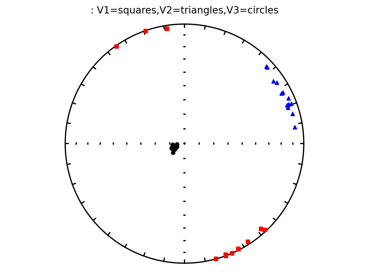
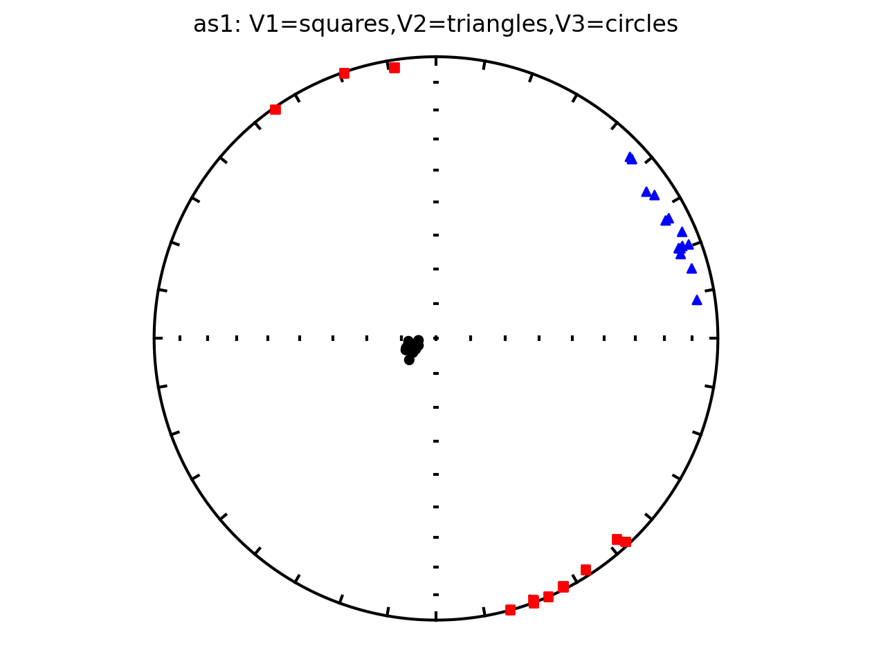
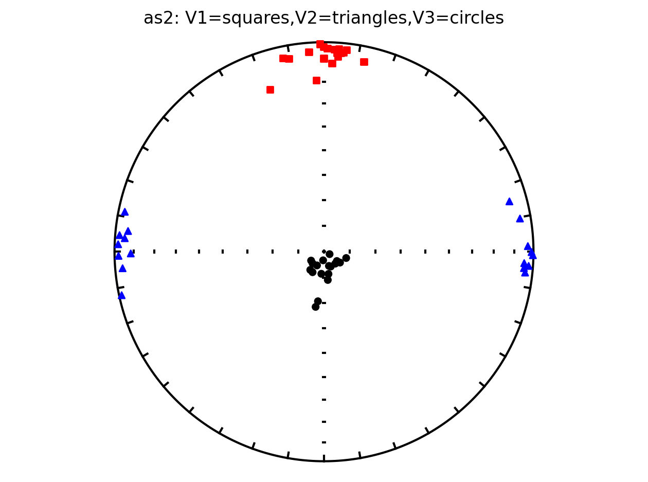
Plot anisotropy tensor by site using ipmag.plot_aniso()

• since the anisotropy tensor data is specimen specific, we will filter for all specimens from the same site and display their results in the same plot

# filter for all specimens within site as1
as1_specimen_data = specimens[specimens['sample'].str.contains('as1')]
as1_specimen_data

	aniso_s	aniso_s_mean	aniso_s_n_measurements	aniso_s_sigma	aniso_s_unit	aniso_type	citations	geologic_classes	geologic_types	lithologies	method_codes	sample	specimen
specimen name
as1a1	0.34406999:0.34145039:0.31447965:-0.00168019:0...	0.000250	15	0.000525	SI	AMS	This study	Sedimentary	Sediment Layer	Shallow Marine Sediments	AE-H:LP-X	as1a	as1a1
as1a2	0.34351686:0.34047559:0.31600755:-0.00129778:0...	0.000229	15	0.000781	SI	AMS	This study	Sedimentary	Sediment Layer	Shallow Marine Sediments	AE-H:LP-X	as1a	as1a2
as1a3	0.34317553:0.34108347:0.315741:-0.00083286:0.0...	0.000235	15	0.000366	SI	AMS	This study	Sedimentary	Sediment Layer	Shallow Marine Sediments	AE-H:LP-X	as1a	as1a3
as1b1	0.34141964:0.34004751:0.31853285:-0.0005353:0....	0.000241	15	0.000546	SI	AMS	This study	Sedimentary	Sediment Layer	Shallow Marine Sediments	AE-H:LP-X	as1b	as1b1
as1b2	0.34097505:0.34068653:0.31833842:-0.00101421:0...	0.000230	15	0.000482	SI	AMS	This study	Sedimentary	Sediment Layer	Shallow Marine Sediments	AE-H:LP-X	as1b	as1b2
as1b3	0.34512332:0.34413338:0.3107433:-0.00177674:0....	0.000254	15	0.000518	SI	AMS	This study	Sedimentary	Sediment Layer	Shallow Marine Sediments	AE-H:LP-X	as1b	as1b3
as1c1	0.3430306:0.34192824:0.31504112:-0.000796:0.00...	0.000264	15	0.000400	SI	AMS	This study	Sedimentary	Sediment Layer	Shallow Marine Sediments	AE-H:LP-X	as1c	as1c1
as1c2	0.34327549:0.34130883:0.31541568:-0.00056881:0...	0.000277	15	0.000762	SI	AMS	This study	Sedimentary	Sediment Layer	Shallow Marine Sediments	AE-H:LP-X	as1c	as1c2
as1c3	0.34189418:0.34063521:0.31747064:-0.00066421:0...	0.000237	15	0.000503	SI	AMS	This study	Sedimentary	Sediment Layer	Shallow Marine Sediments	AE-H:LP-X	as1c	as1c3
as1d1	0.34377083:0.34210697:0.3141222:-0.00068657:0....	0.000263	15	0.000535	SI	AMS	This study	Sedimentary	Sediment Layer	Shallow Marine Sediments	AE-H:LP-X	as1d	as1d1
as1d2	0.34193784:0.34051162:0.31755051:-0.00086076:0...	0.000235	15	0.000579	SI	AMS	This study	Sedimentary	Sediment Layer	Shallow Marine Sediments	AE-H:LP-X	as1d	as1d2
as1d3	0.34405649:0.34288949:0.31305403:-0.00178181:0...	0.000285	15	0.000841	SI	AMS	This study	Sedimentary	Sediment Layer	Shallow Marine Sediments	AE-H:LP-X	as1d	as1d3
as1e1	0.34592408:0.34170985:0.31236601:-0.00087383:0...	0.000285	15	0.000882	SI	AMS	This study	Sedimentary	Sediment Layer	Shallow Marine Sediments	AE-H:LP-X	as1e	as1e1
as1e2	0.34244603:0.34016421:0.31738976:-0.00094397:0...	0.000232	15	0.000480	SI	AMS	This study	Sedimentary	Sediment Layer	Shallow Marine Sediments	AE-H:LP-X	as1e	as1e2

ipmag.plot_aniso(fignum=0, aniso_df=as1_specimen_data ,)

{'data': 0, 'conf': 1}

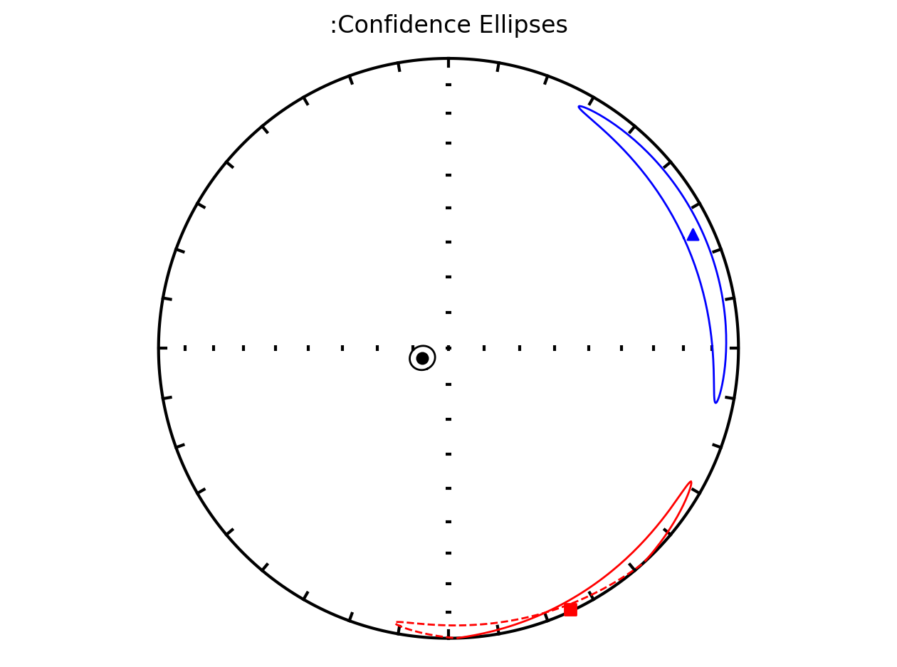
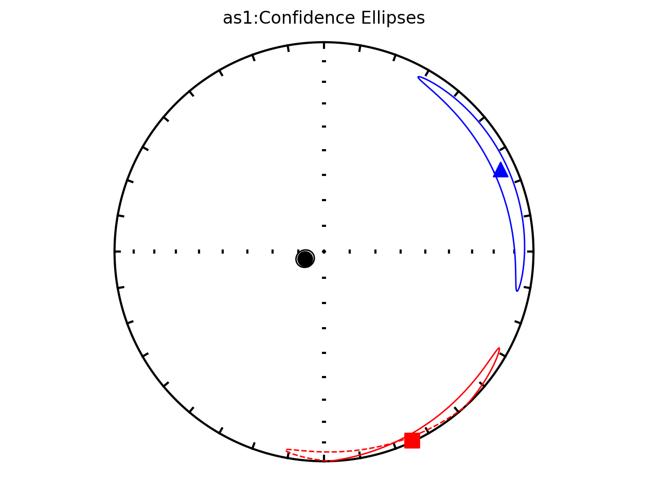
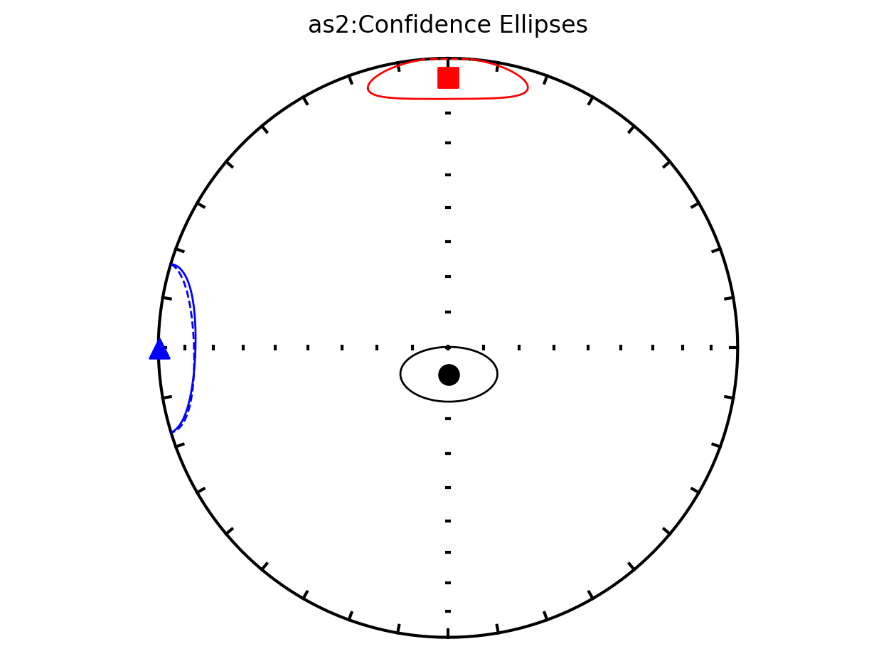
Plot all specimens in the contribution with Hext ellipses

We can also plot all of the AMS data from the study along with the Hext confidence ellipses. This is done by providing our contribution object to the function ipmag.aniso_magic_nb() and setting the parameter ihext=True.

ipmag.aniso_magic_nb(contribution=contribution, 
                     ihext=True,
                     save_plots=False)

(True, [])

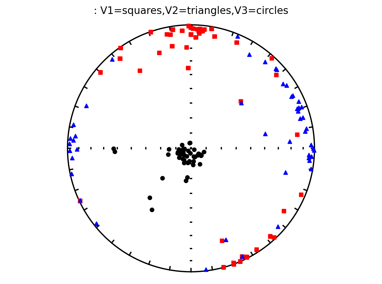
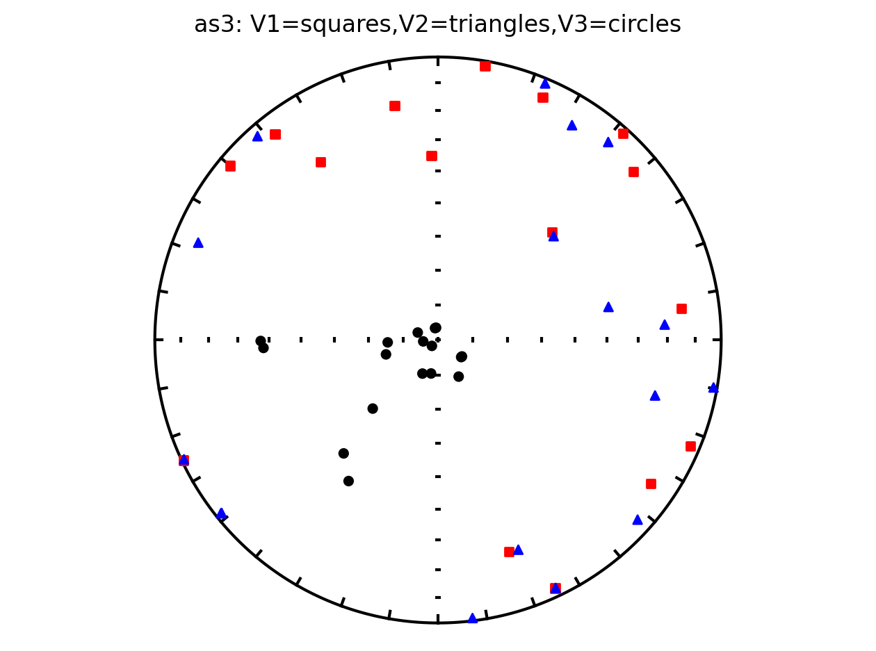
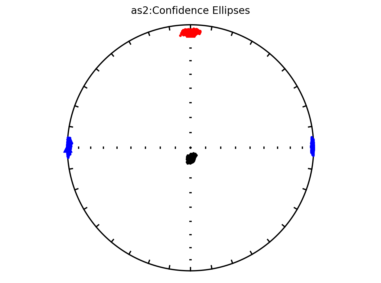
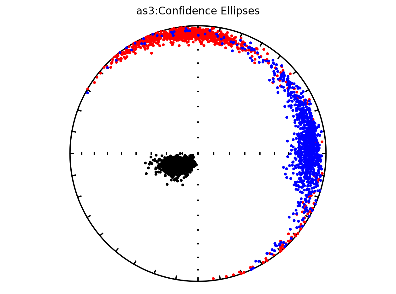
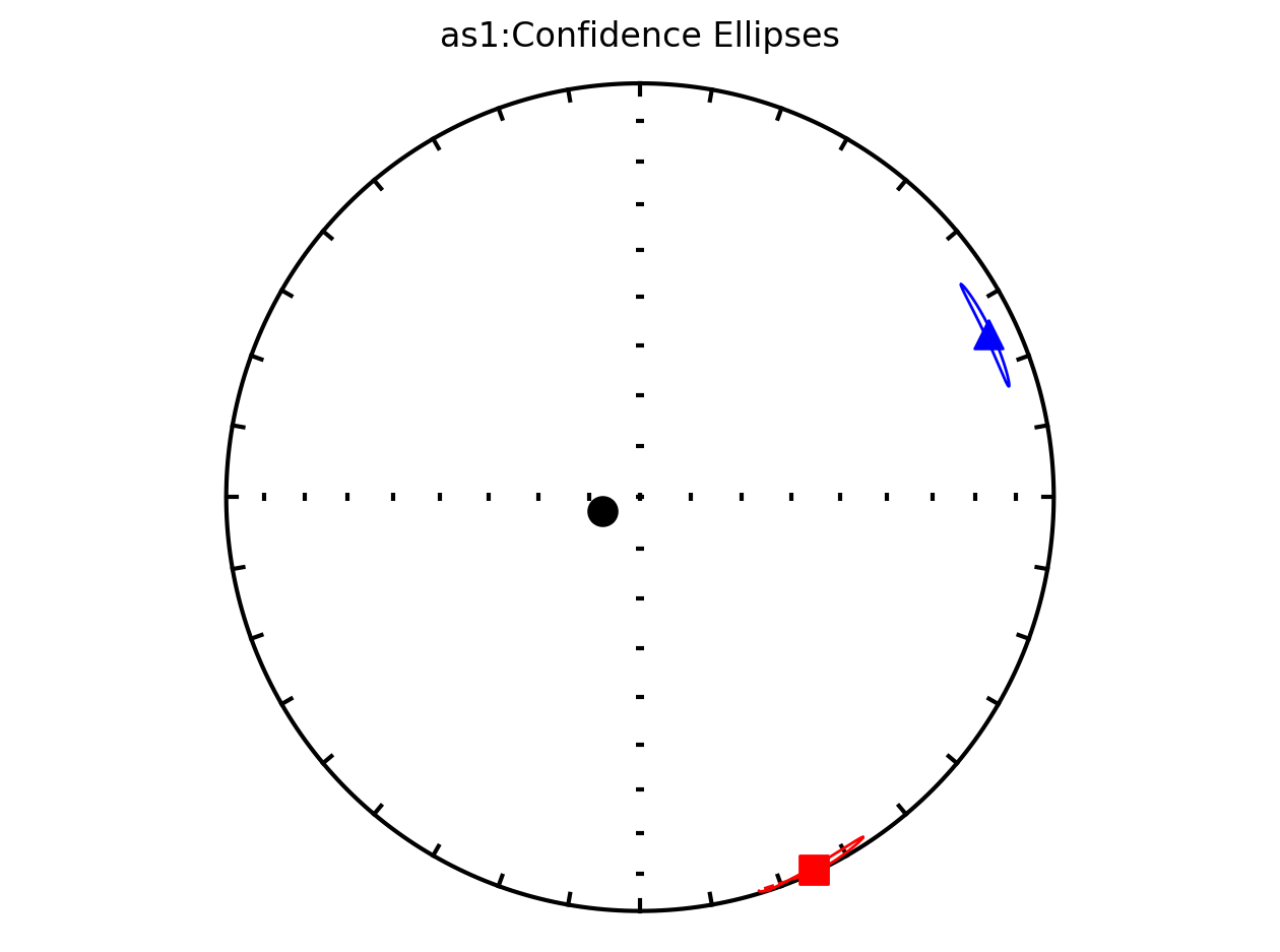
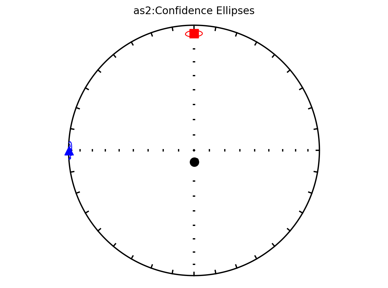
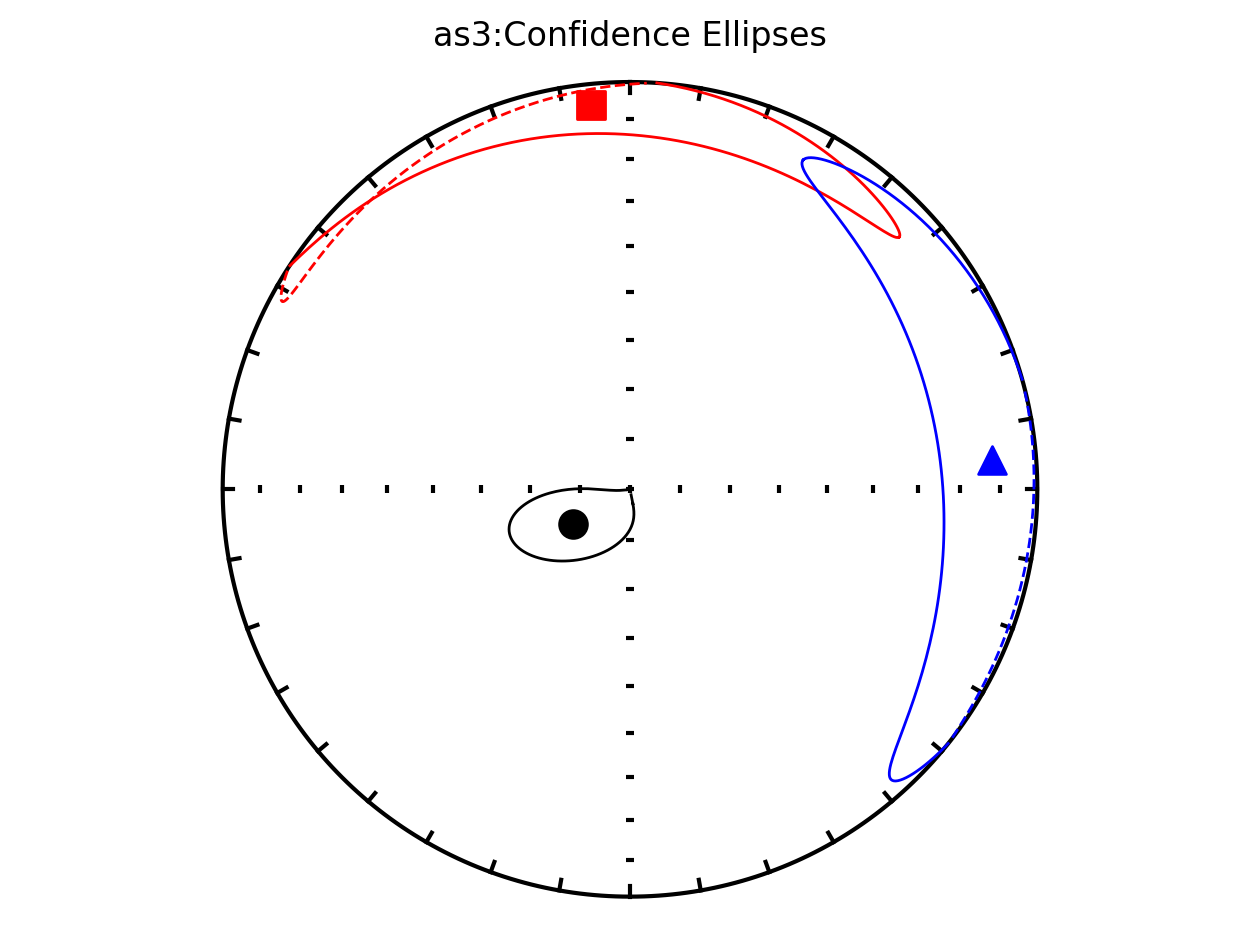
Plot by site with Hext ellipses

The above plot is all of the data from the study. However, in the Schwehr and Tauxe (2003) study the data are from three distinct sites:

• as1; they refer to this site as a cryptoslump and call it site B in the paper

• as2; they refer to this site as a slump and call it site C in the paper

• as3; they refer this cite as undeformed and call it site A in the paper.

It therefore makes sense to plot the data by site since they have distinct behavoirs. We can plot the data by site by setting isite=True. The name of the site will be in the title of the plot.

ipmag.aniso_magic_nb(contribution=contribution, 
                     ihext=True,
                     isite=True,
                     save_plots=False)

(True, [])

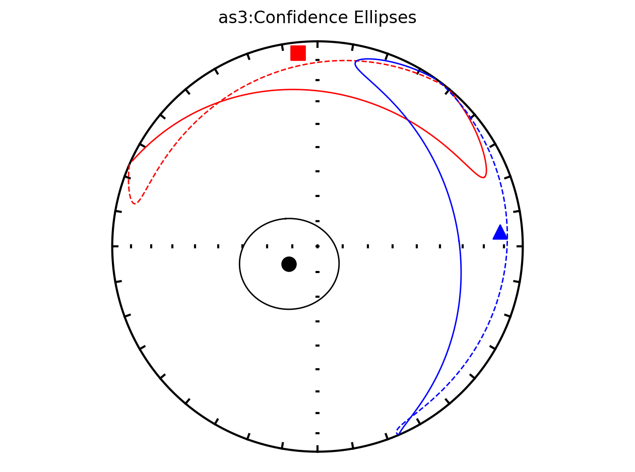
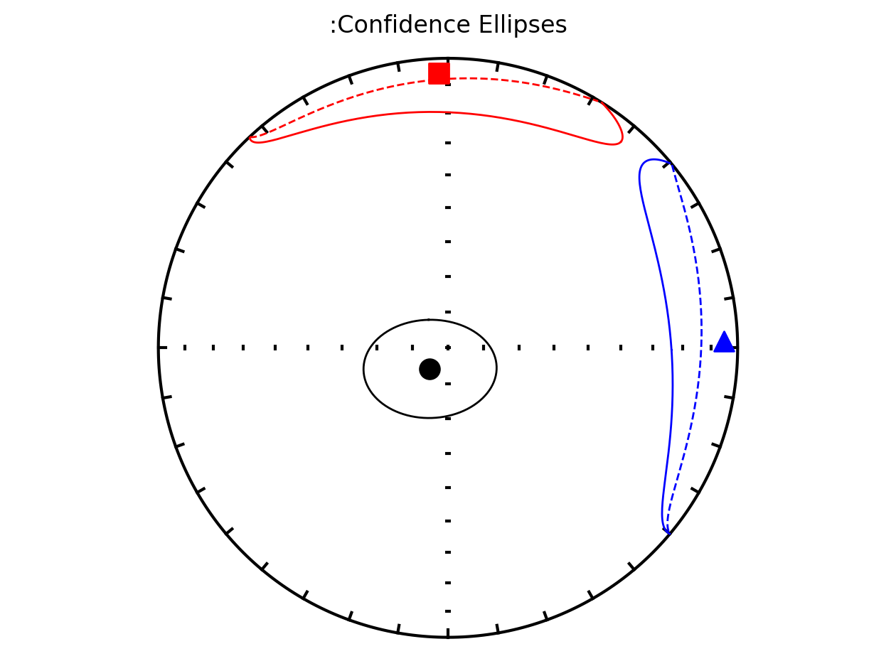
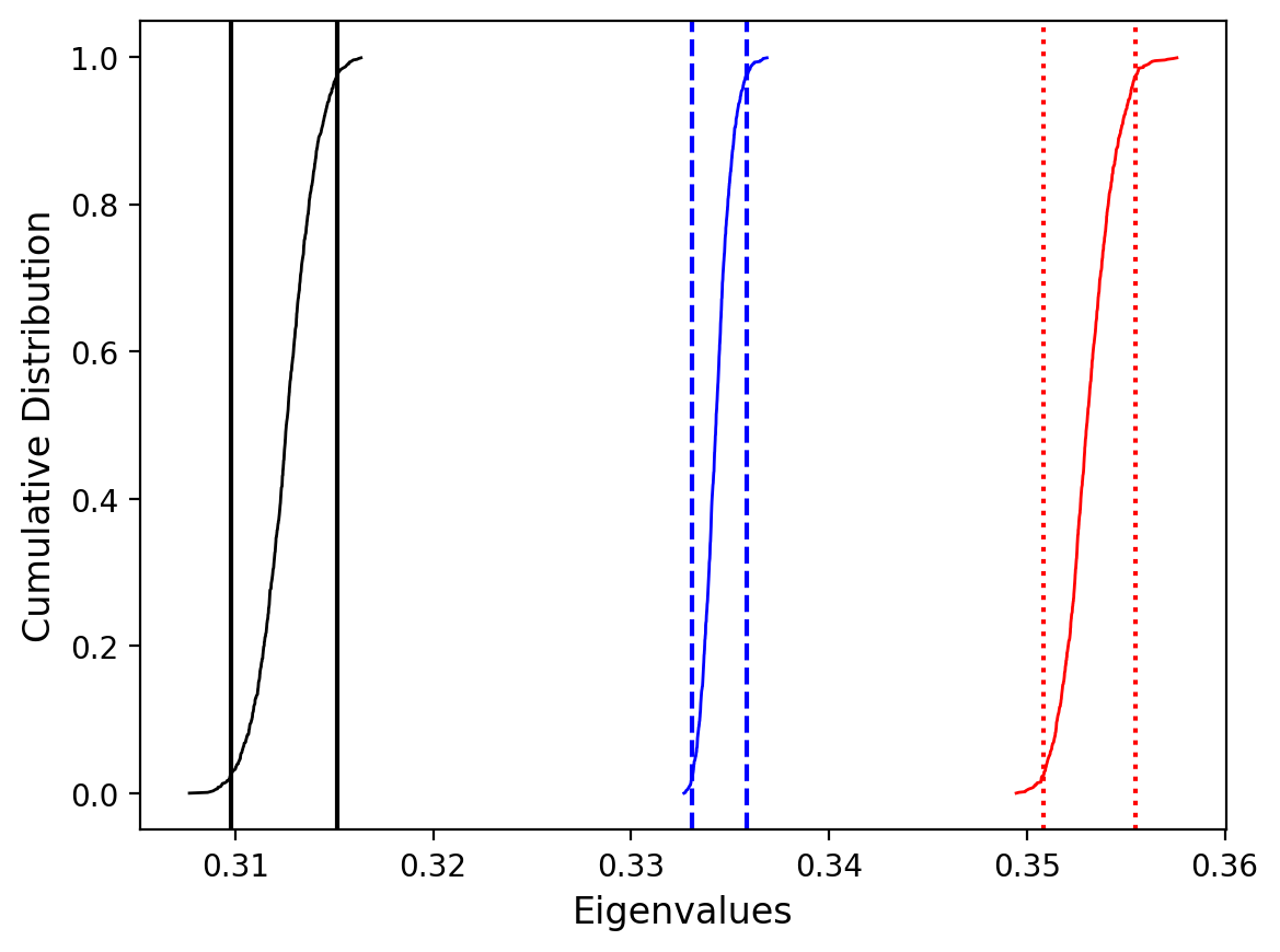
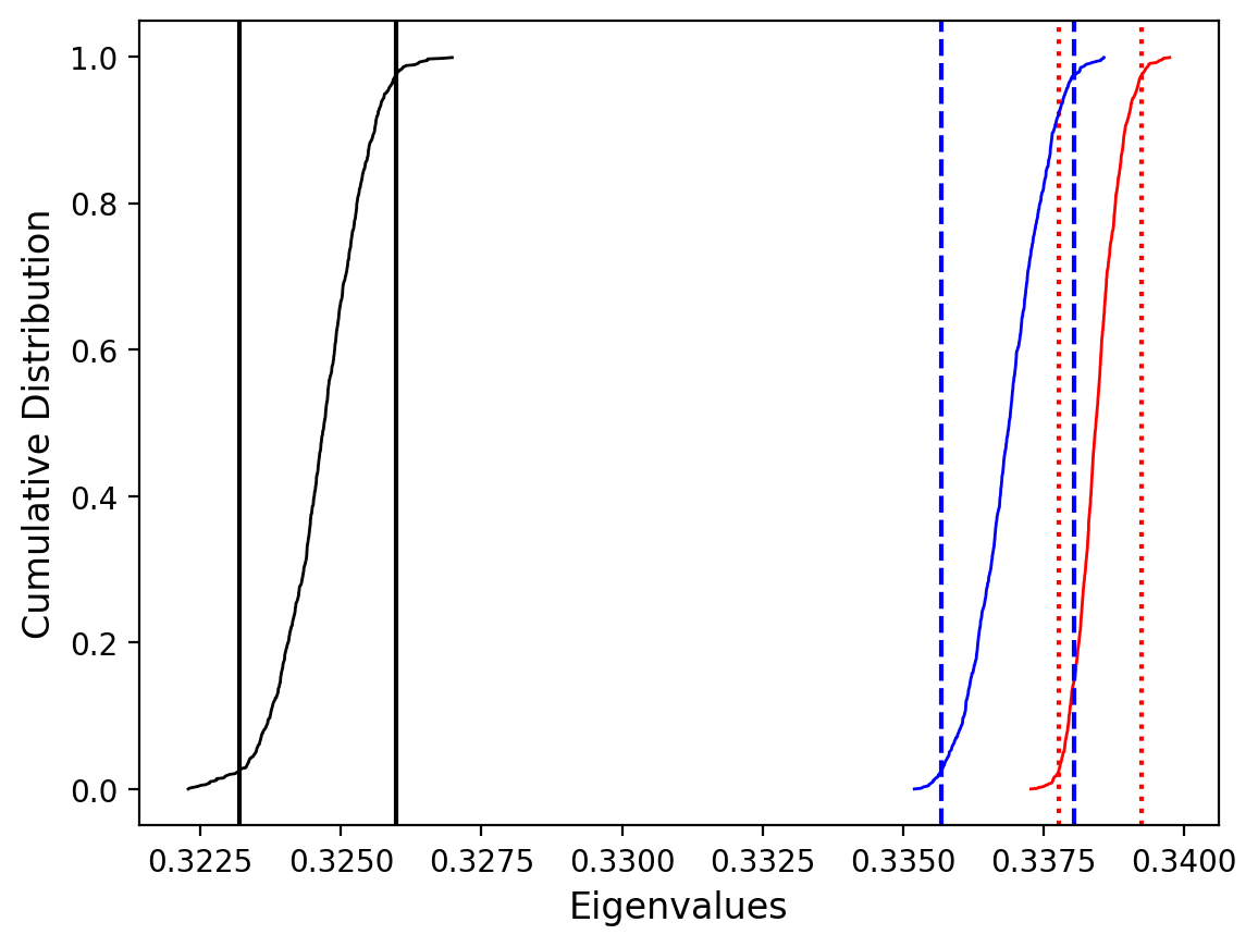
Plot by site with bootstrap uncertainty

Rather than using Hext ellipses, we can generate a plot with bootstrap resamples by setting ivec=True.

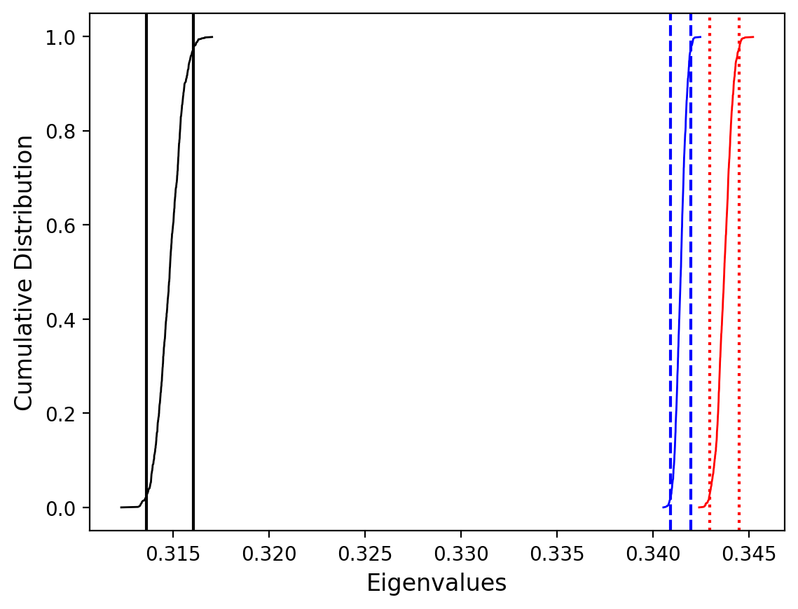
Site as3 (the unslumped sedimentary rocks of Schwehr and Tauxe, 2003) is a nice example of an oblate fabric. Once the code cell below is run, examine it and you will see that the plot of the cumulative distributions mean eigenvalues overlap for \(\tau_1\) and \(\tau_2\) while \(\tau_3\) is significantly smaller. This fabric is characteristic of undeformed sedimentary rocks deposited under the influence of minimal paleocurrents.

ipmag.aniso_magic_nb(contribution=contribution, 
                     ihext=False,
                     iboot=True,
                     isite=True,
                     ivec=True,
                     save_plots=False)

(True, [])

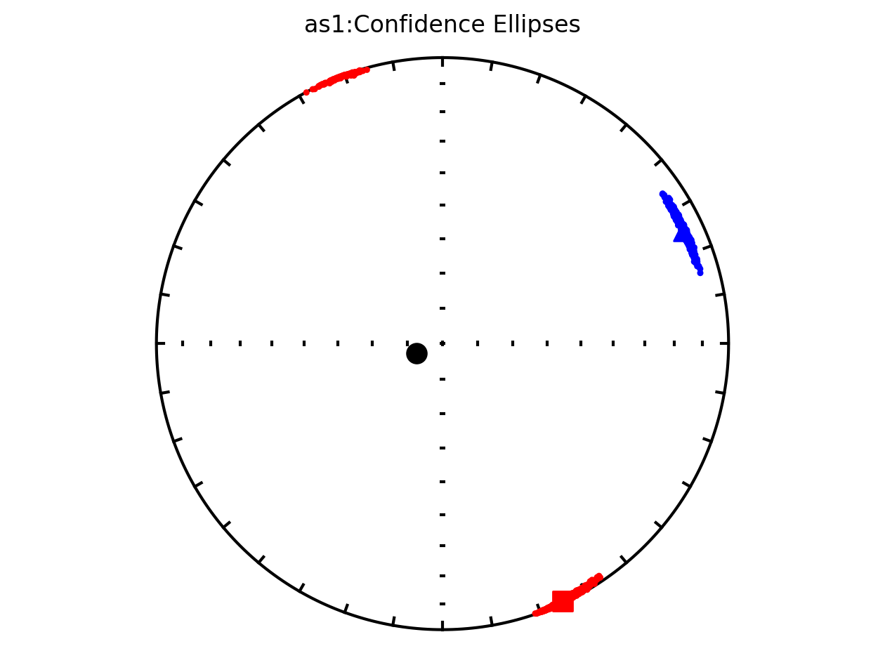
Bootstrap ellipses

In the above plots, the parameter ivec=True resulted in the bootstrap resampled means being shown. Rather than plotting these means, the resulting 95% confidence ellipses associated with the bootstrap approach can be plotted by setting iboot=True and ivec=False. These ellipses are generated for each site in the code cell below.

ipmag.aniso_magic_nb(contribution=contribution, 
                     ihext=False,
                     iboot=True,
                     ivec=False,
                     isite=True,
                     save_plots=False)

(True, [])

Here are all of the parameters that can be used within the ipmag.aniso_magic_nb() function:

• contribution: pmagpy contribution_builder.Contribution object; if not provided will be created in directory (default: None). If provided, infile/samp_file/site_file may be left blank

• infile: Specimens formatted file with aniso_s data (default: ‘specimens.txt’)

• samp_file: Samples formatted file with sample => site relationship (default: ‘samples.txt’)

• site_file: Sites formatted file with site => location relationship (default: ‘sites.txt’)

• verbose: Boolean, if True, print messages to output (default: True)

• ipar: Confidence bound parameter; if True, perform parametric bootstrap - requires non-blank aniso_s_sigma (default: False)

• ihext: Confidence bound parameter; if True, Hext ellipses (default: True)

• ivec: Confidence bound parameter; if True, plot bootstrapped eigenvectors instead of ellipses (default: False)

• isite: Confidence bound parameter; if True, plot by site - requires non-blank samp_file (default: False)

• iboot: Confidence bound parameter; if True, bootstrap ellipses (default: False)

• vec: Eigenvector for comparison with Dir (default: 0)

• Dir: List of [Dec, Inc] for comparison direction (default: [])

• PDir: List of [Pole_dec, Pole_Inc] for pole to plane for comparison; green dots are on the lower hemisphere, cyan are on the upper hemisphere (default: [])

• crd: String, coordinate system for plotting (‘s’ for specimen coordinates, ‘g’ for geographic coordinates, ‘t’ for tilt corrected coordinates) (default: ‘s’)

• num_bootstraps: Integer, number of bootstraps to perform (default: 1000)

• dir_path: String, directory path (default: ‘.’)

• fignum: Integer, matplotlib figure number (default: 1)

• save_plots: Boolean, if True, create and save all requested plots (default: True)

• interactive: Boolean, if True, interactively plot and display for each specimen (default: False)

• fmt: String, format for figures (‘svg’, ‘jpg’, ‘pdf’, ‘png’) (default: ‘png’)