2020 MagIC Workshop PmagPy notebook demo#
Go to the jupyter-hub website at https://jupyterhub.earthref.org/ to run this online. You will have to log in to the earthref website with your ORCID, but then you will have a workspace to use this and the other PmagPy jupyter notebooks.
Alternatively, you can put this notebook in a working directory on your own laptop. You would then have to install Python and the PmagPy software package on your computer (if you have not already done so). The instructions for that are here: https://earthref.org/PmagPy/cookbook/. Follow the instructions for “Full PmagPy install and update” through section 1.4 (Quickstart with PmagPy notebooks). This notebook is in the collection of PmagPy notebooks.
Click on the cell below and then click on ‘Run’ from the menu above to import the desired functionality
# Import PmagPy modules
import pmagpy.pmag as pmag
import pmagpy.pmagplotlib as pmagplotlib
import pmagpy.ipmag as ipmag

# Import plotting modules
has_cartopy, Cartopy = pmag.import_cartopy() # import mapping module, if it is available
import matplotlib.pyplot as plt # our plotting buddy
# This allows you to make matplotlib plots inside the notebook.
%matplotlib inline

# Import more useful modules
import numpy as np # the fabulous NumPy package
import pandas as pd # and  Pandas for data wrangling
import os # some useful operating system functions
from importlib import reload # for reloading module if they get changed after initial import
from IPython.display import Image
import imageio # for making animations
# set up the directory structure for this notebook, if not already present:
dirs=os.listdir() # get a list of directories in this one
if 'MagIC_example_1' not in dirs:
    os.mkdir("MagIC_example_1")
if 'MagIC_example_2' not in dirs:
    os.mkdir("MagIC_example_2")
if 'MagIC_example_3' not in dirs:
    os.mkdir("MagIC_example_3")
Overview of demonstration#
This notebook has three exercises that demonstrate various aspects of the PmagPy software.
Exercise 1 looks at a typical “directional” data set and shows how to make useful plots like the equal area projection, maps of VGPs and basemaps of site locations.
Exercise 2 shows how to get geomagnetic vectors from IGRF-like tables and several ways of looking at the data through time and space.
Exercise 3 considers directional (polarity), anisotropy data and natural gamma radiation (NGR), a measure of the dominance of clay versus diatomaceous ooze in this core, as a function of depth in an IODP core.
When you have worked through these examples, check out the other PmagPy notebooks in the PmagPy software distribution.
Exercise 1#
Hunt around the earthref.org/MagIC/search page for a data set you would like to look at. We will use the data of Behar et al., 2019, DOI: 10.1029/2019GC008479 for this exercise.
Once you have the DOI or the MagIC ID number (which in this case is 16676, there are two ways to download the contribution file: 1) with the MagIC ID (id=16676) using ipmag.download_magic_from_id() and with the DOI using ipmag.download_magic_from_doi().
download the magic contribution file, move it to the directory Example_1, and unpack it with ipmag.download_magic().
Use PmagPy functions to make the following plots:
use ipmag.eqarea_magic() to make an equal area plot
use ipmag.vgpmap_magic() to make a map of VGPs
use ipmag.reversal_test_bootstrap() for a bootstrap reversals test
use pmagplotlib.plot_map() to make a site map
First we need to learn a trick: To understand what a particular PmagPy function expects as input and delivers, use the Python help function
help(ipmag.download_magic_from_id)
Help on function download_magic_from_id in module pmagpy.ipmag:

download_magic_from_id(con_id)
    Download a public contribution matching the provided
    contribution ID from earthref.org/MagIC.

    Parameters
    ----------
    doi : str
        DOI for a MagIC

    Returns
    ---------
    result : bool
    message : str
        Error message if download didn't succeed
Let’s try the contribution ID way first:
dir_path='MagIC_example_1' # set the path to the correct working directory
magic_id='16676' # set the magic ID number
magic_contribution='magic_contribution_'+magic_id+'.txt' # set the file name string
ipmag.download_magic_from_id(magic_id) # download the contribution from MagIC
os.rename(magic_contribution, dir_path+'/'+magic_contribution) # move the contribution to the directory
ipmag.download_magic(magic_contribution,dir_path=dir_path,print_progress=False) # unpack the file
1  records written to file  /Users/ltauxe/Meetings_2020/MagIC_Workshop/MagIC_example_1/contribution.txt
1  records written to file  /Users/ltauxe/Meetings_2020/MagIC_Workshop/MagIC_example_1/locations.txt
91  records written to file  /Users/ltauxe/Meetings_2020/MagIC_Workshop/MagIC_example_1/sites.txt
611  records written to file  /Users/ltauxe/Meetings_2020/MagIC_Workshop/MagIC_example_1/samples.txt
676  records written to file  /Users/ltauxe/Meetings_2020/MagIC_Workshop/MagIC_example_1/specimens.txt
6297  records written to file  /Users/ltauxe/Meetings_2020/MagIC_Workshop/MagIC_example_1/measurements.txt
1  records written to file  /Users/ltauxe/Meetings_2020/MagIC_Workshop/MagIC_example_1/criteria.txt
91  records written to file  /Users/ltauxe/Meetings_2020/MagIC_Workshop/MagIC_example_1/ages.txt
True
Now let’s try to do this with the API for DOIs:
dir_path='MagIC_example_1' # set the path to the correct working directory
reference_doi='10.1029/2019GC008479'
magic_contribution='magic_contribution.txt'
ipmag.download_magic_from_doi(reference_doi)
os.rename(magic_contribution, dir_path+'/'+magic_contribution)
ipmag.download_magic(magic_contribution,dir_path=dir_path,print_progress=False)
16676/magic_contribution_16676.txt extracted to magic_contribution.txt

1  records written to file  /Users/ltauxe/Meetings_2020/MagIC_Workshop/MagIC_example_1/contribution.txt
1  records written to file  /Users/ltauxe/Meetings_2020/MagIC_Workshop/MagIC_example_1/locations.txt
91  records written to file  /Users/ltauxe/Meetings_2020/MagIC_Workshop/MagIC_example_1/sites.txt
611  records written to file  /Users/ltauxe/Meetings_2020/MagIC_Workshop/MagIC_example_1/samples.txt
676  records written to file  /Users/ltauxe/Meetings_2020/MagIC_Workshop/MagIC_example_1/specimens.txt
6297  records written to file  /Users/ltauxe/Meetings_2020/MagIC_Workshop/MagIC_example_1/measurements.txt
1  records written to file  /Users/ltauxe/Meetings_2020/MagIC_Workshop/MagIC_example_1/criteria.txt
91  records written to file  /Users/ltauxe/Meetings_2020/MagIC_Workshop/MagIC_example_1/ages.txt
True
Now we can get to the fun stuff of making plots.
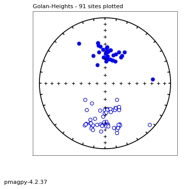
Equal area net example#
use ipmag.eqarea_magic()
# first get help on how to use it:
help(ipmag.eqarea_magic)
Help on function eqarea_magic in module pmagpy.ipmag:

eqarea_magic(in_file='sites.txt', dir_path='.', input_dir_path='', spec_file='specimens.txt', samp_file='samples.txt', site_file='sites.txt', loc_file='locations.txt', plot_by='all', crd='g', ignore_tilt=False, save_plots=True, fmt='svg', contour=False, color_map='coolwarm', plot_ell='', n_plots=5, interactive=False, contribution=None, source_table='sites', image_records=False)
    makes equal area projections from declination/inclination data

    Parameters
    ----------
    in_file : str, default "sites.txt"
    dir_path : str
        output directory, default "."
    input_dir_path : str
        input file directory (if different from dir_path), default ""
    spec_file : str
        input specimen file name, default "specimens.txt"
    samp_file: str
        input sample file name, default "samples.txt"
    site_file : str
        input site file name, default "sites.txt"
    loc_file : str
        input location file name, default "locations.txt"
    plot_by : str
        [spc, sam, sit, loc, all] (specimen, sample, site, location, all), default "all"
    crd : ['s','g','t'], coordinate system for plotting whereby:
        s : specimen coordinates, aniso_tile_correction = -1
        g : geographic coordinates, aniso_tile_correction = 0 (default)
        t : tilt corrected coordinates, aniso_tile_correction = 100
    ignore_tilt : bool
        default False.  If True, data are unoriented (allows plotting of measurement dec/inc)
    save_plots : bool
        plot and save non-interactively, default True
    fmt : str
        ["png", "svg", "pdf", "jpg"], default "svg"
    contour : bool
        plot as color contour
    colormap : str
        color map for contour plotting, default "coolwarm"
        see cartopy documentation for more options
    plot_ell : str
        [F,K,B,Be,Bv] plot Fisher, Kent, Bingham, Bootstrap ellipses or Bootstrap eigenvectors
        default "" plots none
    n_plots : int
        maximum number of plots to make, default 5
        if you want to make all possible plots, specify "all"
    interactive : bool, default False
        interactively plot and display for each specimen
        (this is best used on the command line or in the Python interpreter)
    contribution : cb.Contribution, default None
        if provided, use Contribution object instead of reading in
        data from files
    source_table : table to get plot data from (only needed with contribution argument)
        for example, you could specify source_table="measurements" and plot_by="sites"
        to plot measurement data by site.
        default "sites"
    image_records : generate and return a record for each image in a list of dicts
        which can be ingested by pmag.magic_write
        bool, default False


    Returns
    ---------
    if image_records == False:
        type - Tuple : (True or False indicating if conversion was successful, file name(s) written)
    if image_records == True:
       Tuple : (True or False indicating if conversion was successful, output file name written, list of image recs)
# now we do it for real:
ipmag.eqarea_magic(dir_path=dir_path,save_plots=False)
-I- Using online data model
-I- Getting method codes from earthref.org
-I- Importing controlled vocabularies from https://earthref.org
-W- File /Users/ltauxe/Meetings_2020/MagIC_Workshop/MagIC_example_1/criteria.txt is incomplete and will be ignored
91  sites records read in
All
(True, [])
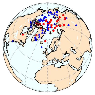
Map of VGPs#
use ipmag.vgpmap_magic() to plot the VGPs from the same data
# get help message for vgpmap_magic
help(ipmag.vgpmap_magic)
Help on function vgpmap_magic in module pmagpy.ipmag:

vgpmap_magic(dir_path='.', results_file='sites.txt', crd='', sym='ro', size=8, rsym='g^', rsize=8, fmt='pdf', res='c', proj='ortho', flip=False, anti=False, fancy=False, ell=False, ages=False, lat_0=0, lon_0=0, save_plots=True, interactive=False, contribution=None, image_records=False)
    makes a map of vgps and a95/dp,dm for site means in a sites table

    Parameters
    ----------
    dir_path : str, default "."
        input directory path
    results_file : str, default "sites.txt"
        name of MagIC format sites file
    crd : str, default ""
       coordinate system [g, t] (geographic, tilt_corrected)
    sym : str, default "ro"
        symbol color and shape, default red circles
        (see matplotlib documentation for more color/shape options)
    size : int, default 8
        symbol size
    rsym : str, default "g^"
        symbol for plotting reverse poles
        (see matplotlib documentation for more color/shape options)
    rsize : int, default 8
        symbol size for reverse poles
    fmt : str, default "pdf"
        format for figures, ["svg", "jpg", "pdf", "png"]
    res : str, default "c"
        resolution [c, l, i, h] (crude, low, intermediate, high)
    proj : str, default "ortho"
        ortho = orthographic
        lcc = lambert conformal
        moll = molweide
        merc = mercator
    flip : bool, default False
        if True, flip reverse poles to normal antipode
    anti : bool, default False
        if True, plot antipodes for each pole
    fancy : bool, default False
        if True, plot topography (not yet implemented)
    ell : bool, default False
        if True, plot ellipses
    ages : bool, default False
        if True, plot ages
    lat_0 : float, default 0.
        eyeball latitude
    lon_0 : float, default 0.
        eyeball longitude
    save_plots : bool, default True
        if True, create and save all requested plots
    interactive : bool, default False
       if True, interactively plot and display
        (this is best used on the command line only)
    image_records : bool, default False
        if True, return a list of created images

    Returns
    ---------
    if image_records == False:
        type - Tuple : (True or False indicating if conversion was successful, file name(s) written)
    if image_records == True:
       Tuple : (True or False indicating if conversion was successful, output file name written, list of image recs)
dir_path='MagIC_example_1' # set the path to your working directory
ipmag.vgpmap_magic(dir_path=dir_path,size=50,flip=True,save_plots=False,lat_0=60,rsym='b^',rsize=50)
'table_column' <class 'KeyError'>
-W- File /Users/ltauxe/Meetings_2020/MagIC_Workshop/MagIC_example_1/criteria.txt is missing required information
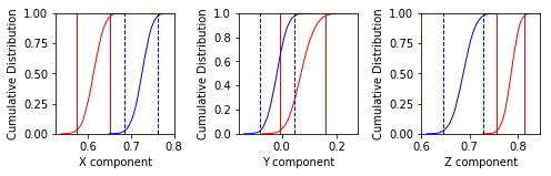
Bootstrap reversals test#
use ipmag.reversal_test_bootstrap() to do the reversals test
help(ipmag.reversal_test_bootstrap)
Help on function reversal_test_bootstrap in module pmagpy.ipmag:

reversal_test_bootstrap(dec=None, inc=None, di_block=None, plot_stereo=False, save=False, save_folder='.', fmt='svg')
    Conduct a reversal test using bootstrap statistics (Tauxe, 2010) to
    determine whether two populations of directions could be from an antipodal
    common mean.

    Parameters
    ----------
    dec: list of declinations
    inc: list of inclinations
        or
    di_block: a nested list of [dec,inc]
        A di_block can be provided in which case it will be used instead of
        dec, inc lists.

    plot_stereo : before plotting the CDFs, plot stereonet with the
        bidirectionally separated data (default is False)
    save : boolean argument to save plots (default is False)
    save_folder : directory where plots will be saved (default is current directory, '.')
    fmt : format of saved figures (default is 'svg')

    Returns
    -------
    plots : Plots of the cumulative distribution of Cartesian components are
        shown as is an equal area plot if plot_stereo = True

    Examples
    --------
    Populations of roughly antipodal directions are developed here using
    ``ipmag.fishrot``. These directions are combined into a single di_block
    given that the function determines the principal component and splits the
    data accordingly by polarity.

    >>> directions_n = ipmag.fishrot(k=20, n=30, dec=5, inc=-60)
    >>> directions_r = ipmag.fishrot(k=35, n=25, dec=182, inc=57)
    >>> directions = directions_n + directions_r
    >>> ipmag.reversal_test_bootstrap(di_block=directions, plot_stereo = True)

    Data can also be input to the function as separate lists of dec and inc.
    In this example, the di_block from above is split into lists of dec and inc
    which are then used in the function:

    >>> direction_dec, direction_inc, direction_moment = ipmag.unpack_di_block(directions)
    >>> ipmag.reversal_test_bootstrap(dec=direction_dec,inc=direction_inc, plot_stereo = True)
# read in the data into a Pandas DataFrame
dir_path='MagIC_example_1' # set the path to your working directory
sites_df=pd.read_csv(dir_path+'/sites.txt',sep='\t',header=1)
# pick out the declinations and inclinations
decs=sites_df.dir_dec.values
incs=sites_df.dir_inc.values
# call the function
ipmag.reversal_test_bootstrap(dec=decs,inc=incs,plot_stereo=False)
Make a site map#
use pmagplotlib.plot_map() to make a site map
help(pmagplotlib.plot_map)
Help on function plot_map in module pmagpy.pmagplotlib:

plot_map(fignum, lats, lons, Opts)
    makes a cartopy map  with lats/lons
    Requires installation of cartopy

    Parameters:
    _______________
    fignum : matplotlib figure number
    lats : array or list of latitudes
    lons : array or list of longitudes
    Opts : dictionary of plotting options:
        Opts.keys=
            proj : projection [supported cartopy projections:
                pc = Plate Carree
                aea = Albers Equal Area
                aeqd = Azimuthal Equidistant
                lcc = Lambert Conformal
                lcyl = Lambert Cylindrical
                merc = Mercator
                mill = Miller Cylindrical
                moll = Mollweide [default]
                ortho = Orthographic
                robin = Robinson
                sinu = Sinusoidal
                stere = Stereographic
                tmerc = Transverse Mercator
                utm = UTM [set zone and south keys in Opts]
                laea = Lambert Azimuthal Equal Area
                geos = Geostationary
                npstere = North-Polar Stereographic
                spstere = South-Polar Stereographic
            latmin : minimum latitude for plot
            latmax : maximum latitude for plot
            lonmin : minimum longitude for plot
            lonmax : maximum longitude
            lat_0 : central latitude
            lon_0 : central longitude
            sym : matplotlib symbol
            symsize : symbol size in pts
            edge : markeredgecolor
            cmap : matplotlib color map
            res :  resolution [c,l,i,h] for low/crude, intermediate, high
            boundinglat : bounding latitude
            sym : matplotlib symbol for plotting
            symsize : matplotlib symbol size for plotting
            names : list of names for lats/lons (if empty, none will be plotted)
            pltgrd : if True, put on grid lines
            padlat : padding of latitudes
            padlon : padding of longitudes
            gridspace : grid line spacing
            global : global projection [default is True]
            oceancolor : 'azure'
            landcolor : 'bisque' [choose any of the valid color names for matplotlib
              see https://matplotlib.org/examples/color/named_colors.html
            details : dictionary with keys:
                coasts : if True, plot coastlines
                rivers : if True, plot rivers
                states : if True, plot states
                countries : if True, plot countries
                ocean : if True, plot ocean
                lakes : if True, plot lakes
                fancy : if True, plot etopo 20 grid
                    NB:  etopo must be installed
        if Opts keys not set :these are the defaults:
           Opts={'latmin':-90,'latmax':90,'lonmin':0,'lonmax':360,'lat_0':0,'lon_0':0,'proj':'moll','sym':'ro,'symsize':5,'edge':'black','pltgrid':1,'res':'c','boundinglat':0.,'padlon':0,'padlat':0,'gridspace':30,'details':all False,'edge':None,'cmap':'jet','fancy':0,'zone':'','south':False,'oceancolor':'azure','landcolor':'bisque'}
NB: the most recent PmagPy version fixes the scale issue - but it is SLOW at high resolution… so set Opts[‘res’] to ‘c’ for crude for a quick look. if you want to be dazzled - set it to ‘h’ but be prepared to wait for a while… ‘i’ for intermediate is probably good enough for most purposes (50m resolution)
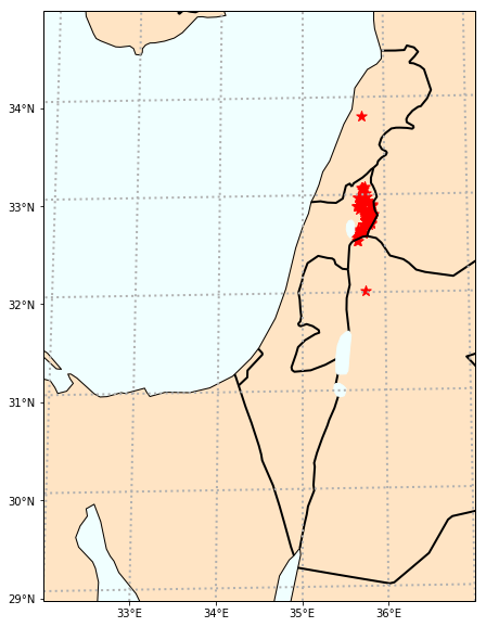
dir_path='MagIC_example_1' # set the path to your working directory
# read in the data file:
site_df=pd.read_csv(dir_path+'/sites.txt',sep='\t',header=1)
# pick out the longitudes and latitudes
lons=site_df['lon'].values
lats=site_df['lat'].values
# set some options
Opts={}
Opts['sym']='r*' # sets the symbol to white dots
Opts['symsize']=100 # sets symbol size to 3 pts
Opts['proj']='lcc' # Lambert Conformal projection
Opts['pltgrid']=True
Opts['lat_0']=33
Opts['lon_0']=35
Opts['latmin']=29
Opts['latmax']=35
Opts['lonmin']=32
Opts['lonmax']=37
Opts['gridspace']=1
Opts['details']={}
Opts['details']['coasts']=True
Opts['details']['ocean']=True
Opts['details']['countries']=True
Opts['global']=False
Opts['res']='i'
plt.figure(1,(10,10)) # optional - make a map

pmagplotlib.plot_map(1, lats, lons, Opts)
Exercise 2:#
use pmag.pinc() to calculate the GAD inclination for a particular latitude (e.g., 33)
use ipmag.igrf() and ipmag.igrf_print() to get values of the field for a specific place (e.g., San Diego at lon=-117,lat=33,alt=0) and date (2019)
make a plot of declination, inclination, B for a specific place and range of dates
use pmag.do_mag_map() and pmagplotlib.plot_mag_map() to make a map of the field at a specific date (2019)
make a movie of the field for the last 1000 years using the cals10k.2 model of Constable et al. (2016)
help(pmag.pinc)
Help on function pinc in module pmagpy.pmag:

pinc(lat)
    calculate paleoinclination from latitude using dipole formula: tan(I) = 2tan(lat)
    Parameters
    ________________

    lat : either a single value or an array of latitudes

    Returns
    -------

    array of inclinations
gad_inc=pmag.pinc(33)
print(gad_inc)
52.406157522519074
help(ipmag.igrf)
Help on function igrf in module pmagpy.ipmag:

igrf(input_list, mod='', ghfile='')
    Determine Declination, Inclination and Intensity from the IGRF model.
    (http://www.ngdc.noaa.gov/IAGA/vmod/igrf.html)

    Parameters
    ----------
    input_list : list with format [Date, Altitude, Latitude, Longitude]
        date must be in decimal year format XXXX.XXXX (Common Era)
        altitude is in kilometers
    mod :  desired model
        "" : Use the IGRF
        custom : use values supplied in ghfile
        or choose from this list
        ['arch3k','cals3k','pfm9k','hfm10k','cals10k.2','cals10k.1b']
        where:
            arch3k (Korte et al., 2009)
            cals3k (Korte and Constable, 2011)
            cals10k.1b (Korte et al., 2011)
            pfm9k  (Nilsson et al., 2014)
            hfm10k is the hfm.OL1.A1 of Constable et al. (2016)
            cals10k.2 (Constable et al., 2016)
            the first four of these models, are constrained to agree
            with gufm1 (Jackson et al., 2000) for the past four centuries


    gh : path to file with l m g h data

    Returns
    -------
    igrf_array : array of IGRF values (0: dec; 1: inc; 2: intensity (in nT))

    Examples
    --------
    >>> local_field = ipmag.igrf([2013.6544, .052, 37.87, -122.27])
    >>> local_field
    array([  1.39489916e+01,   6.13532008e+01,   4.87452644e+04])
    >>> ipmag.igrf_print(local_field)
    Declination: 13.949
    Inclination: 61.353
    Intensity: 48745.264 nT
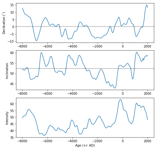
date,lat,lon,alt=2019.9,33,-117,0 # set variables for ipmag.igrf
local=ipmag.igrf([date, alt, lat, lon]) # get the local field vector
ipmag.igrf_print(local) # format for nice printing
Declination: 11.376
Inclination: 58.140
Intensity: 46239.890 nT
mod='cals10k.2' # set model to Constable et al. (2016) cals10k.2
lat,lon,alt=33,-117,0  # set location information
gad_inc=pmag.pinc(lat) # get the GAD inclination at the latitude
dates=range(-8000,2050,50) # get a list of desired dates
local_vectors=[] # make a container to put the vectors in
for d in dates: # step through the date list
    local=ipmag.igrf([d, alt, lat, lon],mod=mod) # get the vector at that place and time
    local_vectors.append([d,local[0],local[1],local[2]]) # append it to the container of field vectors
df=pd.DataFrame(local_vectors,columns=['Date','Dec','Inc','B_nT']) # make a Pandas DataFrame
df['B_uT']=df['B_nT']*1e-3 # convert from nanotesla to microtesla
df.loc[df['Dec']>180,'Dec']=df['Dec']-360. # make declinations centered around 0
fig=plt.figure(1,(8,8)) # make a figure object
ax1=fig.add_subplot(311) # add subplots (3 rows, one column, plot 1)
ax2=fig.add_subplot(312) # plot 2
ax3=fig.add_subplot(313) # plot 3
ax1.plot(df['Date'],df['Dec']) # plot declination against date
ax1.axhline(0,color='black',linestyle='dotted') # make a horizontal black line at 0
ax2.plot(df['Date'],df['Inc']) # plot inclination against date
ax2.axhline(gad_inc,color='black',linestyle='dotted')
ax3.plot(df['Date'],df['B_uT']) # plot microtesla against date
ax1.set_ylabel(r'Declination ($^{\circ}$)') # y label on plot 1
ax2.set_ylabel('Inclination')# y label on plot 2
ax3.set_ylabel('Intensity')# y label on plot 3
ax3.set_xlabel('Age (+/- AD)'); # x label on bottom plot (3)
help(pmag.do_mag_map)
Help on function do_mag_map in module pmagpy.pmag:

do_mag_map(date, lon_0=0, alt=0, file='', mod='cals10k', resolution='low')
    returns lists of declination, inclination and intensities for lat/lon grid for
    desired model and date.

    Parameters:
    _________________
    date = Required date in decimal years (Common Era, negative for Before Common Era)

    Optional Parameters:
    ______________
    mod  = model to use ('arch3k','cals3k','pfm9k','hfm10k','cals10k.2','shadif14k','cals10k.1b','custom')
    file = l m g h formatted filefor custom model
    lon_0 : central longitude for Hammer projection
    alt  = altitude
    resolution = ['low','high'] default is low

    Returns:
    ______________
    Bdec=list of declinations
    Binc=list of inclinations
    B = list of total field intensities in nT
    Br = list of radial field intensities
    lons = list of longitudes evaluated
    lats = list of latitudes evaluated
help(pmagplotlib.plot_mag_map)
Help on function plot_mag_map in module pmagpy.pmagplotlib:

plot_mag_map(fignum, element, lons, lats, element_type, cmap='coolwarm', lon_0=0, date='', contours=False, proj='PlateCarree')
    makes a color contour map of geomagnetic field element

    Parameters
    ____________
    fignum : matplotlib figure number
    element : field element array from pmag.do_mag_map for plotting
    lons : longitude array from pmag.do_mag_map for plotting
    lats : latitude array from pmag.do_mag_map for plotting
    element_type : [B,Br,I,D] geomagnetic element type
        B : field intensity
        Br : radial field intensity
        I : inclinations
        D : declinations
    Optional
    _________
    contours : plot the contour lines on top of the heat map if True
    proj : cartopy projection ['PlateCarree','Mollweide']
           NB: The Mollweide projection can only be reliably with cartopy=0.17.0; otherwise use lon_0=0.  Also, for declinations, PlateCarree is recommended.
    cmap : matplotlib color map - see https://matplotlib.org/examples/color/colormaps_reference.html for options
    lon_0 : central longitude of the Mollweide projection
    date : date used for field evaluation,
           if custom ghfile was used, supply filename

    Effects
    ______________
    plots a color contour map with  the desired field element
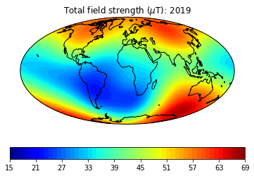
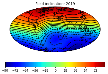
# define some useful parameters
date,mod,lon_0,alt,ghfile=2019,'cals10k.2',0,0,"" # only date is required
Ds,Is,Bs,Brs,lons,lats=pmag.do_mag_map(date,mod=mod,lon_0=lon_0,alt=alt,file=ghfile) # get the global data
help(pmagplotlib.plot_mag_map)
Help on function plot_mag_map in module pmagpy.pmagplotlib:

plot_mag_map(fignum, element, lons, lats, element_type, cmap='coolwarm', lon_0=0, date='', contours=False, proj='PlateCarree', min=20, max=80)
    makes a color contour map of geomagnetic field element

    Parameters
    ____________
    fignum : matplotlib figure number
    element : field element array from pmag.do_mag_map for plotting
    lons : longitude array from pmag.do_mag_map for plotting
    lats : latitude array from pmag.do_mag_map for plotting
    element_type : [B,Br,I,D] geomagnetic element type
        B : field intensity
        Br : radial field intensity
        I : inclinations
        D : declinations
    Optional
    _________
    contours : plot the contour lines on top of the heat map if True
    proj : cartopy projection ['PlateCarree','Mollweide']
           NB: The Mollweide projection can only be reliably with cartopy=0.17.0; otherwise use lon_0=0.  Also, for declinations, PlateCarree is recommended.
    cmap : matplotlib color map - see https://matplotlib.org/examples/color/colormaps_reference.html for options
    lon_0 : central longitude of the Mollweide projection
    date : date used for field evaluation,
           if custom ghfile was used, supply filename
    min : float or int
        minimum value for the color bar
    max : float or int
        maximum value for the color bar

    Effects
    ______________
    plots a color contour map with  the desired field element
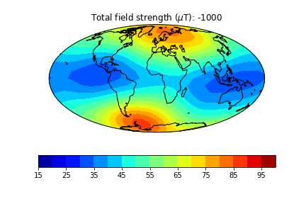
cmap='jet' # nice color map for contourf
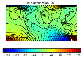
pmagplotlib.plot_mag_map(1,Bs,lons,lats,'B',cmap=cmap,date=date,proj='Mollweide',contours=False) # plot the field strength
pmagplotlib.plot_mag_map(2,Is,lons,lats,'I',cmap=cmap,date=date,proj='Mollweide',contours=True)# plot the inclination
pmagplotlib.plot_mag_map(3,Ds,lons,lats,'D',cmap=cmap,date=date,contours=True);# plot the declination
This part of the exercise will create a movie from a bunch of .png files. To do a high resolution movie takes too much time, especially when there are many people logged onto the jupyter-hub web site. So we will just illustrate how it is done, then tantalize you with a higher resolution movie that you are free to make as you will. on your own computer or after the workshop.
dir_path='MagIC_example_2' # set the directory path name
files=os.listdir(dir_path) # get a list of the directory
for f in files:
if '.png' in f:os.remove(dir_path+'/'+f) # delete all the existing .png files in that directory
mod,lon_0,alt,ghfile='cals10k.2',0,0,"" # define the variables
cmap,title='jet','Intensity' # nice color map for contourf
fignum=1
dates=range(-1000,2100,500) # make maps for these years.
# to make a high resolution, smooth movie, uncomment this line
#dates=range(-1000,2100,50) # make maps for these years.
lon_0=0 # center the maps at the Greenwich meridian
element='B' # let's do field strength
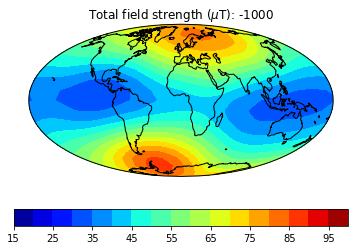
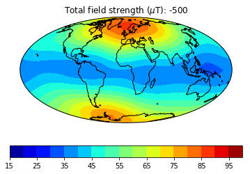
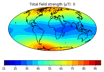
for date in dates: # step through the loop
Ds,Is,Bs,Brs,lons,lats=pmag.do_mag_map(date,mod=mod,lon_0=lon_0,alt=alt,file=ghfile)
pmagplotlib.plot_mag_map(fignum,Bs,lons,lats,'B',cmap=cmap,date=date,proj='Mollweide',
min=15,max=100,contours=False) # plot the field strength
figstr=str(fignum)
while len(figstr)<4:figstr='0'+figstr
plt.savefig(dir_path+'/' +title.strip()+'_'+figstr+'.png') # saves the figure. to a folder
fignum+=1
print ('figure saved as: ',title.strip()+'_'+figstr+'.png')
figure saved as:  Intensity_0001.png
figure saved as:  Intensity_0002.png
figure saved as:  Intensity_0003.png
figure saved as:  Intensity_0004.png
figure saved as:  Intensity_0005.png
figure saved as:  Intensity_0006.png
figure saved as:  Intensity_0007.png
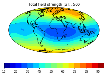
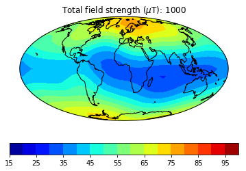
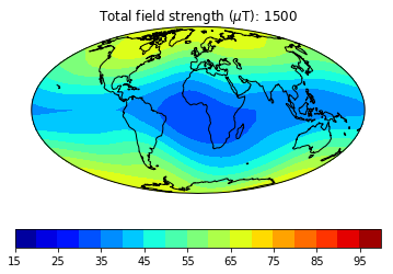
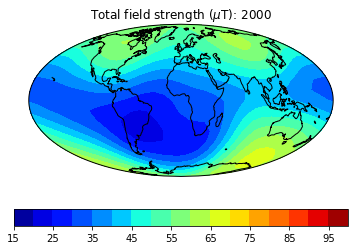
Now we can make the animated gif from these png files
filenames=sorted(os.listdir('MagIC_example_2/')) # listing of the directory
images = [] # make a container to put the image files in
for file in filenames: # step through all the maps
    if '.png' in file: # skip some of the nasty hidden files
        filename='MagIC_example_2/'+file # make filename from the folder name and the file name
        images.append(imageio.imread(filename)) # read it in and stuff in the container
kargs={ 'duration':.3} # .2 second delay between frames
imageio.mimsave('MagIC_example_2/Bmovie.gif', images,'GIF',**kargs) # save to an animated gif.
Image(filename="MagIC_example_2/Bmovie.gif")

Here is an example of one done at higher temporal resolution. You can do this too if you have the patience (perhaps not when dozens of other folks are using the jupyter-hub at the same time!
just uncomment this line in the map making code cell above:
dates=range(-1000,2100,50) # make maps for these years.
Image(filename="MagIC_example_2/BigMovie.gif")
Exercise 3#
download the data from Tauxe et al. (2015; DOI: 10.1016/J.EPSL.2014.12.034; MagIC id:16749) using the wget.download command as in Exercise 1.
Move the downloaded data file to a directory called ‘MagIC_example_3’
Unpack it with ipmag.download_magic()
make a figure with these elements for the interval 40 m to 160 m:
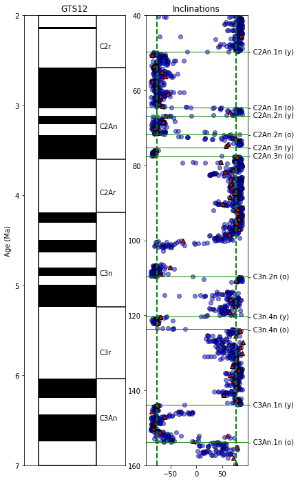
magstrat time scale plot from 2 to 7 Ma
inclinations (dir_inc) from the 20mT step in the measurements table against composite_depth as blue dots
inclinations (dir_inc) from the specimens table against composite depth as red triangles.
put on dotted lines for the GAD inclination
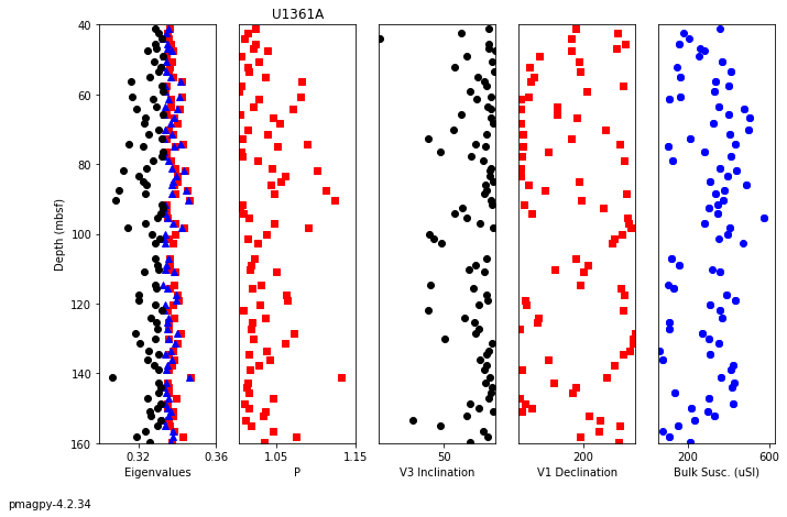
use ipmag.ani_depthplot to plot the anisotropy data against depth in the Hole.
Download and unpack the data#
dir_path='MagIC_example_3' # set the path to your working directory
depth_min, depth_max= 40, 160 # set the core depth bounds as required
# First get the file from MagIC into your working directory:
magic_id='16761'
magic_contribution='magic_contribution_'+magic_id+'.txt' # set the file name string
ipmag.download_magic_from_id(magic_id) # download the contribution from MagIC
os.rename(magic_contribution, dir_path+'/'+magic_contribution) # move the contribution to the directory
ipmag.download_magic(magic_contribution,dir_path=dir_path,print_progress=False) # unpack the file
1  records written to file  /Users/ltauxe/PmagPy/MagIC_example_3/contribution.txt
1  records written to file  /Users/ltauxe/PmagPy/MagIC_example_3/locations.txt
5943  records written to file  /Users/ltauxe/PmagPy/MagIC_example_3/sites.txt
2436  records written to file  /Users/ltauxe/PmagPy/MagIC_example_3/samples.txt
2573  records written to file  /Users/ltauxe/PmagPy/MagIC_example_3/specimens.txt
4697  records written to file  /Users/ltauxe/PmagPy/MagIC_example_3/measurements.txt
60  records written to file  /Users/ltauxe/PmagPy/MagIC_example_3/ages.txt
True
Magstrat figure#
read in the data file as a Pandas DataFrame with pd.read_csv().
All MagIC .txt files are tab delimited. This is indicated with a sep=’\t’ keywork.
The column headers in the second row, hence (because Python counts from zero), header=1
the depth of a particular specimen/site in MagIC is stored in the sites.txt table. You will have to merge the data from that table into the specimens/measurements tables. To do that you need to do a few things:
you need a common key. Because the specimen/sample/site names are the same for an IODP record, make a column in the specimen/measurements dataframes labled ‘site’ that is the same as the specimen.
merge the two dataframes (sites and specimens/measurements) with pd.merge()
dir_path='MagIC_example_3' # set the path to your working directory
depth_min, depth_max= 40, 160 # set the core depth bounds as required
# read in the required data tables:
meas_df=pd.read_csv(dir_path+'/measurements.txt',sep='\t',header=1)
site_df=pd.read_csv(dir_path+'/sites.txt',sep='\t',header=1)
spec_df=pd.read_csv(dir_path+'/specimens.txt',sep='\t',header=1)
ages_df=pd.read_csv(dir_path+'/ages.txt',sep='\t',header=1)
# filter the ages table for method codes that indicate paleomagnetic reversals:
ages_df=ages_df[ages_df['method_codes'].str.contains('PMAG')]
# filter the measurements for the 20 mT (.02 T) step
meas_df.dropna(subset=['treat_ac_field'],inplace=True)
meas_20mT=meas_df[meas_df['treat_ac_field']==0.02]
# make the site key in the measurements and specimens dataframes
meas_20mT['site']=meas_20mT['specimen']
spec_df['site']=spec_df['specimen']
# we only want the core depth out of the sites dataframe, so we can pare it down like this:
depth_df=site_df[['site','core_depth']]
# merge the specimen, depth dataframes
spec_df=pd.merge(spec_df,depth_df,on='site')
# merge the measurements, depth dataframes
meas_20mT=pd.merge(meas_20mT,depth_df,on='site')
# filter for the desired depth range:
spec_df=spec_df[(spec_df['core_depth']>depth_min)&(spec_df['core_depth']<depth_max)]
meas_20mT=meas_20mT[(meas_20mT['core_depth']>depth_min)&(meas_20mT['core_depth']<depth_max)]
# note that the age table has only height (not depth), so these numbers are the opposite
ages_df=ages_df[(ages_df['tiepoint_height']<-depth_min)&(ages_df['tiepoint_height']>-depth_max)]
# get the site latitude (there is only one)
lat=site_df['lat'].unique()[0]
fig=plt.figure(1,(9,12)) # make the figure
ax1=fig.add_subplot(131) # make the first of three subplots
pmagplotlib.plot_ts(ax1,2,7,timescale='gts12') # plot on the time scale
ax2=fig.add_subplot(132) # make the second of three subplots
plt.plot(meas_20mT.dir_inc,meas_20mT.core_depth,'bo',markeredgecolor='black',alpha=.5)
plt.plot(spec_df.dir_inc,spec_df.core_depth,'r^',markeredgecolor='black')

plt.ylim(depth_max,depth_min)
# calculate the geocentric axial dipole field for the site latitude
gad=pmag.pinc(lat) # tan (I) = 2 tan (lat)
# put it on the plot as a green dashed line
plt.axvline(gad,color='green',linestyle='dashed',linewidth=2)
plt.axvline(-gad,color='green',linestyle='dashed',linewidth=2)
plt.title('Inclinations')
pmagplotlib.label_tiepoints(ax2,100,ages_df.tiepoint.values,-1*ages_df.tiepoint_height.values,lines=True)
#
“Christmas tree” of anisotropy#
use ipmag.ani_depthplot()
help(ipmag.ani_depthplot)
Help on function ani_depthplot in module pmagpy.ipmag:

ani_depthplot(spec_file='specimens.txt', samp_file='samples.txt', meas_file='measurements.txt', site_file='sites.txt', age_file='', sum_file='', fmt='svg', dmin=-1, dmax=-1, depth_scale='core_depth', dir_path='.', contribution=None)
    returns matplotlib figure with anisotropy data plotted against depth
    available depth scales: 'composite_depth', 'core_depth' or 'age' (you must provide an age file to use this option).
    You must provide valid specimens and sites files, and either a samples or an ages file.
    You may additionally provide measurements and a summary file (csv).

    Parameters
    ----------
    spec_file : str, default "specimens.txt"
    samp_file : str, default "samples.txt"
    meas_file : str, default "measurements.txt"
    site_file : str, default "sites.txt"
    age_file : str, default ""
    sum_file : str, default ""
    fmt : str, default "svg"
        format for figures, ["svg", "jpg", "pdf", "png"]
    dmin : number, default -1
        minimum depth to plot (if -1, default to plotting all)
    dmax : number, default -1
        maximum depth to plot (if -1, default to plotting all)
    depth_scale : str, default "core_depth"
        scale to plot, ['composite_depth', 'core_depth', 'age'].
        if 'age' is selected, you must provide an ages file.
    dir_path : str, default "."
        directory for input files
    contribution : cb.Contribution, default None
        if provided, use Contribution object instead of reading in
        data from files

    Returns
    ---------
    plot : matplotlib plot, or False if no plot could be created
    name : figure name, or error message if no plot could be created
ipmag.ani_depthplot(dir_path=dir_path,dmin=40,dmax=160);
-I- Using online data model
-I- Getting method codes from earthref.org
-I- Importing controlled vocabularies from https://earthref.org
Plotting External Results#
ipmag.ani_depthplot() reads in a specimen file with the column aniso_s filled in and calculates the eigenvalues for you. in this exercise, you learn to calculate anisotropy eigenvalues from the aniso_s column in the specimens table yourself,
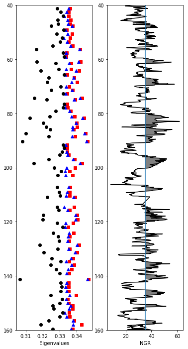
plot anisotropy eigenvalues and the natural gamma radiation values from U1361A between 40 and 160 meters below sea floor
dir_path='MagIC_example_3' # set the path to your working directory
depth_min, depth_max= 40, 160 # set the core depth bounds as required
# read in the data files and filter for desired columns
site_df=pd.read_csv(dir_path+'/sites.txt',sep='\t',header=1)
site_df=site_df[['site','core_depth','external_results']]

anis_df=pd.read_csv(dir_path+'/specimens.txt',sep='\t',header=1)
anis_df['site']=anis_df['specimen']
anis_df.dropna(subset=['aniso_v1'],inplace=True)
# merge with sites and filter for the depth
anis_df=pd.merge(anis_df,site_df,on='site')
anis_df=anis_df[(anis_df.core_depth>depth_min)&(anis_df.core_depth<depth_max)]


# unpack the eigenparameters from aniso_v1,aniso_v2 and aniso_v3 and pick out the eigenvalues
anis_df['tau1']=anis_df['aniso_v1'].str.split(':',expand=True)[0].astype('float').values
anis_df['tau2']=anis_df['aniso_v2'].str.split(':',expand=True)[0].astype('float').values
anis_df['tau3']=anis_df['aniso_v3'].str.split(':',expand=True)[0].astype('float').values

# unpack external results data
site_df['ngr']=site_df['external_results'].str.split(':',expand=True)[1].astype('float').values

# make the plots


fig=plt.figure(1,(6,12)) # make the figure
ax1=fig.add_subplot(121) # make the first of two subplots
ax2=fig.add_subplot(122) # make the second of two subplots

# plot the eigenvalues with the usual symbols
ax1.plot(anis_df['tau1'],anis_df['core_depth'],'rs') # red square
ax1.plot(anis_df['tau2'],anis_df['core_depth'],'b^') # blue triangle
ax1.plot(anis_df['tau3'],anis_df['core_depth'],'ko') # black circle
ax1.set_ylim(depth_max,depth_min) # set the y axis limits
ax1.set_xlabel('Eigenvalues')

# plot the ngr data as a black line
ax2.plot(site_df['ngr'],site_df['core_depth'],'k-')
ax2.set_ylim(depth_max,depth_min) # set the y axis limits
# shade in the high NGR regions - these are the clay dominated layers with higher anisotropy
y2=np.ones(len(site_df['ngr']))*site_df['ngr'].median()
plt.fill_betweenx(site_df['core_depth'],site_df['ngr'], y2,\
                  where = site_df['ngr']>=y2, facecolor='grey')
ax2.axvline(site_df['ngr'].median()) # draw a vertical line up the median values
ax2.set_xlabel('NGR'); # label the X axis