Inspecting directional data in a MagIC contribution using PmagPy#
This template notebook enables inspection of the data within a MagIC contribution. We want to get the data from MagIC, import the data into our notebook, and inspect the data by making plots.
Import functions from PmagPy#
To start with, let’s import some functions from PmagPy:
import pmagpy.ipmag as ipmag
import pandas as pd
import matplotlib.pyplot as plt

%matplotlib inline
%config InlineBackend.figure_format='retina'
Import the data#
We can use ipmag to go download the data from MagIC for us. We can do this in a couple of ways. One way is to use the doi and the function ipmag.download_magic_from_doi(). The other is to use the MagIC contribution ID number with the ipmag.download_magic_from_id() function. Let’s take the id download approach for the study:
Stelten, Thomas, Pivarunas, and Champion (2023). Spatio-temporal clustering of post-caldera eruptions at Yellowstone caldera: implications for volcanic hazards and pre-eruptive magma reservoir configuration. Bulletin of Volcanology 85 (10). doi:10.1007/S00445-023-01665-W.
We can use the MagIC ID of 19640 for this paper which can be replaced with that of another study in the MagIC database.
doi = '10.1007/S00445-023-01665-W'
id = '19640'
directory = './inspecting_MagIC_data/'
result, magic_file_name = ipmag.download_magic_from_id(id, directory = directory)
Running this function will download a file called magic_contribution_19640.txt in the folder that this notebook is in.
In the above code cell, we saved a variable magic_file_name that is the name of the files that was downloaded.
magic_file_name
'./inspecting_MagIC_data/magic_contribution.txt'
Unpacking the tables#
A MagIC contribution is a single .txt file that comprises a number of tables. In the case of this contribution, we have these tables:
ages
contribution
locations
measurements
samples
sites
specimens
We want unpack the contribution into these distinct tables.
ipmag.unpack_magic(magic_file_name, dir_path=directory, print_progress=False)
1  records written to file  /Users/unimos/0000_Github/PmagPy-docs/example_notebooks/template_notebooks/inspecting_MagIC_data/contribution.txt
4  records written to file  /Users/unimos/0000_Github/PmagPy-docs/example_notebooks/template_notebooks/inspecting_MagIC_data/locations.txt
7  records written to file  /Users/unimos/0000_Github/PmagPy-docs/example_notebooks/template_notebooks/inspecting_MagIC_data/sites.txt
71  records written to file  /Users/unimos/0000_Github/PmagPy-docs/example_notebooks/template_notebooks/inspecting_MagIC_data/samples.txt
178  records written to file  /Users/unimos/0000_Github/PmagPy-docs/example_notebooks/template_notebooks/inspecting_MagIC_data/specimens.txt
1247  records written to file  /Users/unimos/0000_Github/PmagPy-docs/example_notebooks/template_notebooks/inspecting_MagIC_data/measurements.txt
4  records written to file  /Users/unimos/0000_Github/PmagPy-docs/example_notebooks/template_notebooks/inspecting_MagIC_data/ages.txt
True
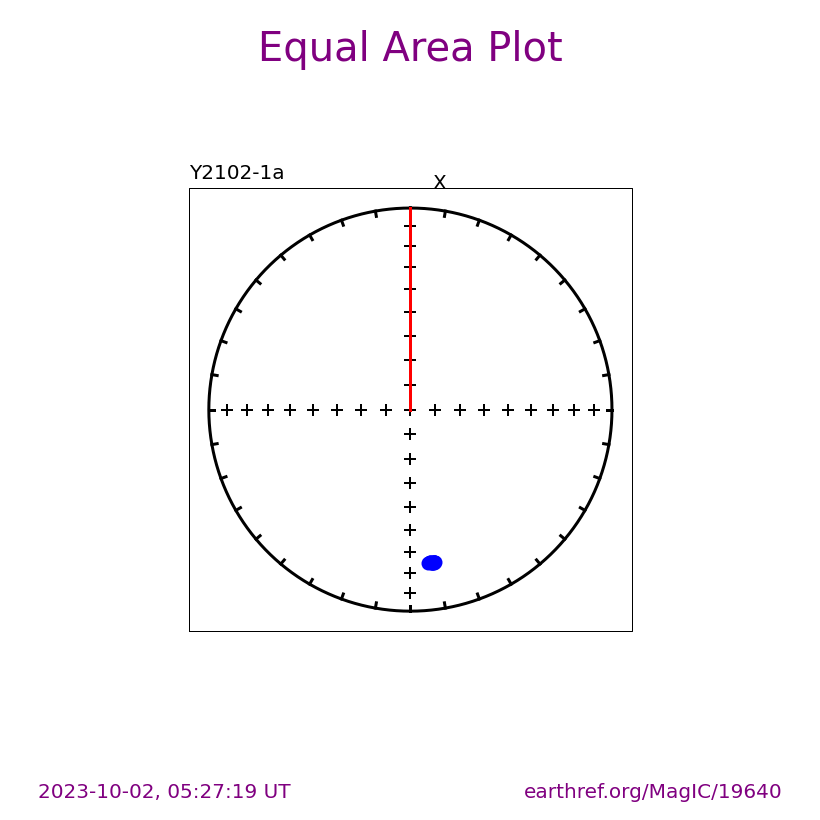
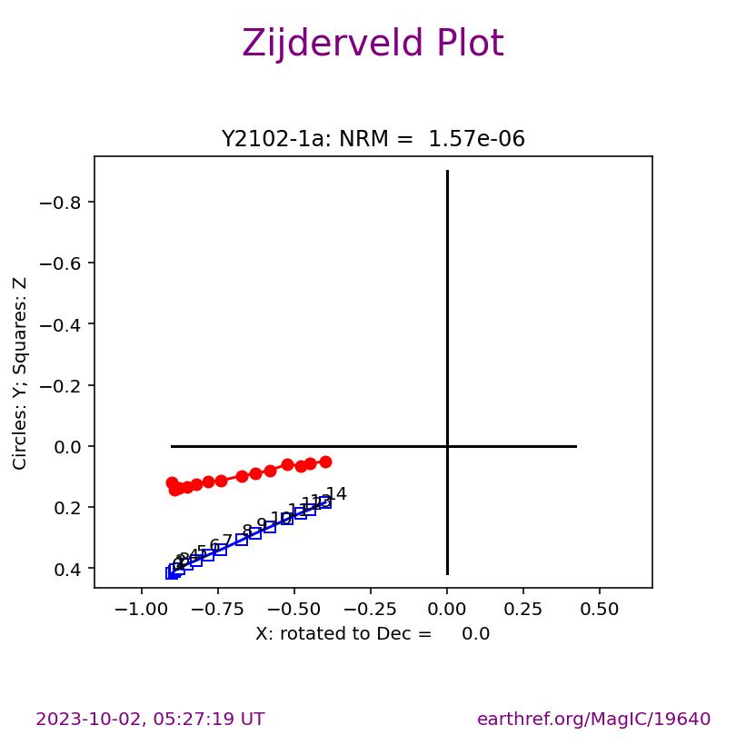
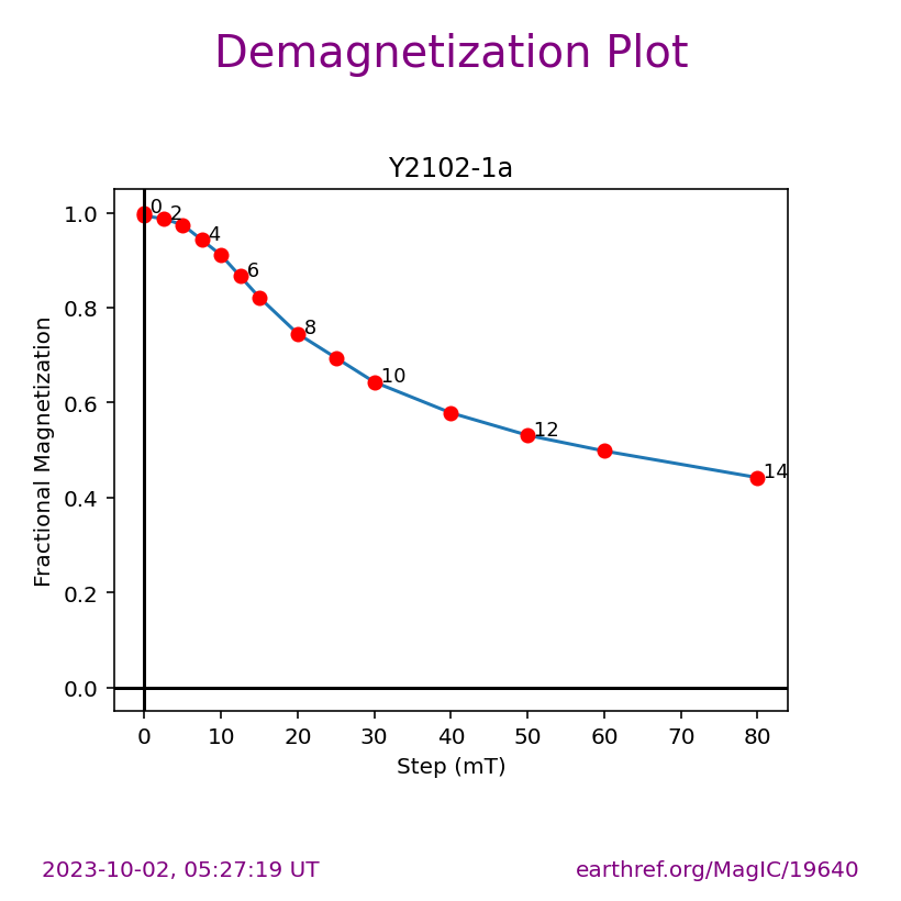
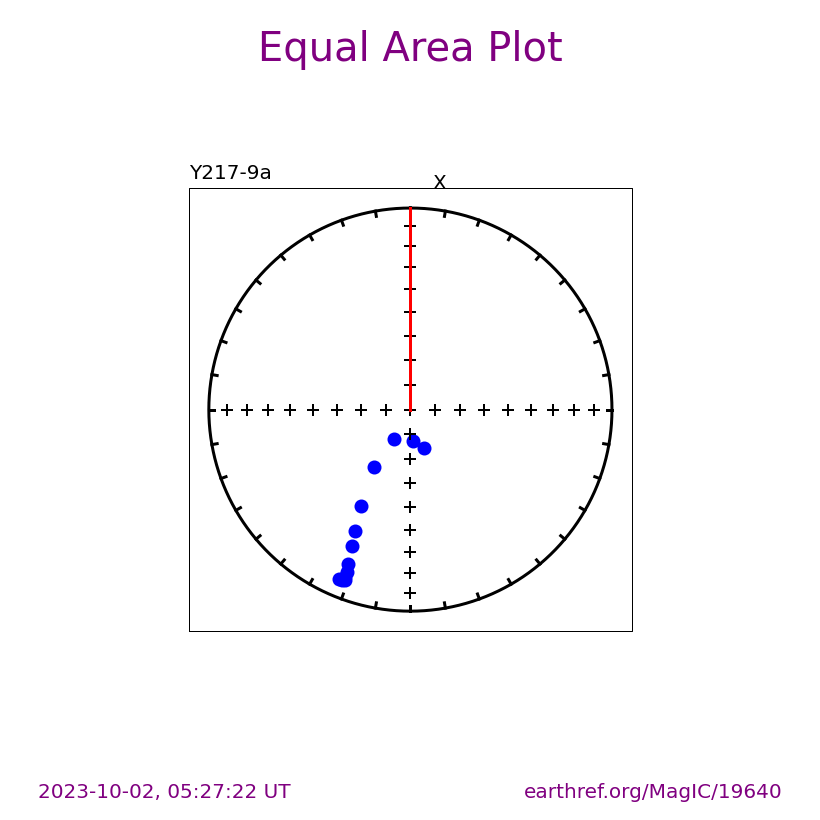
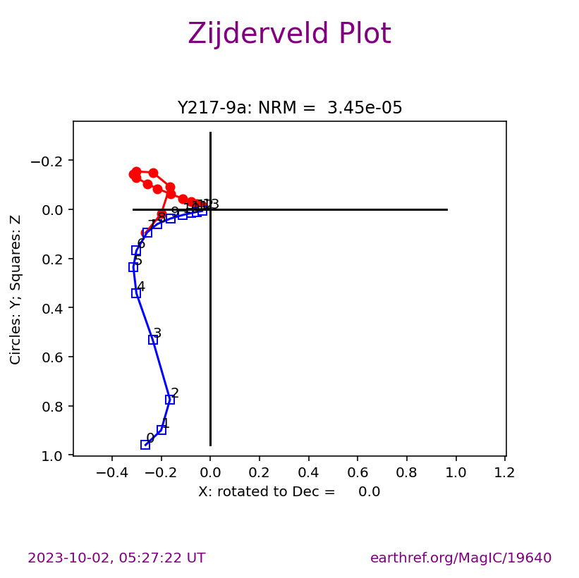
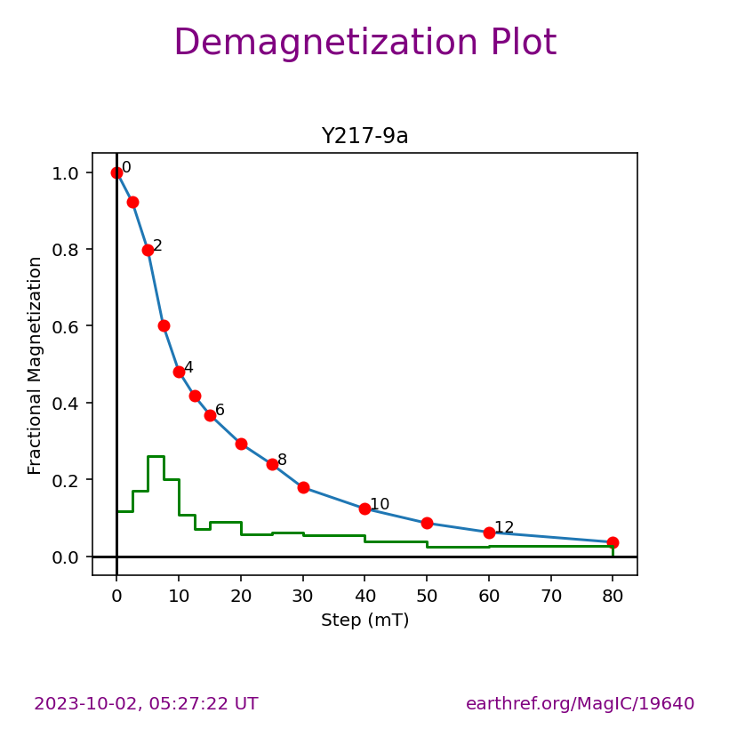
Visualizing measurement level data#
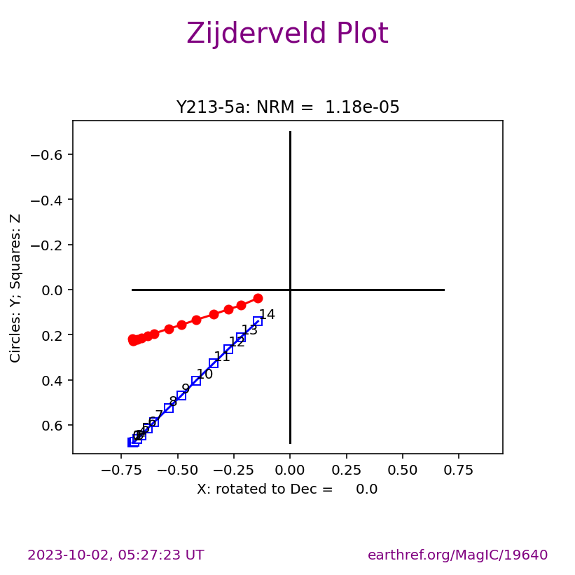
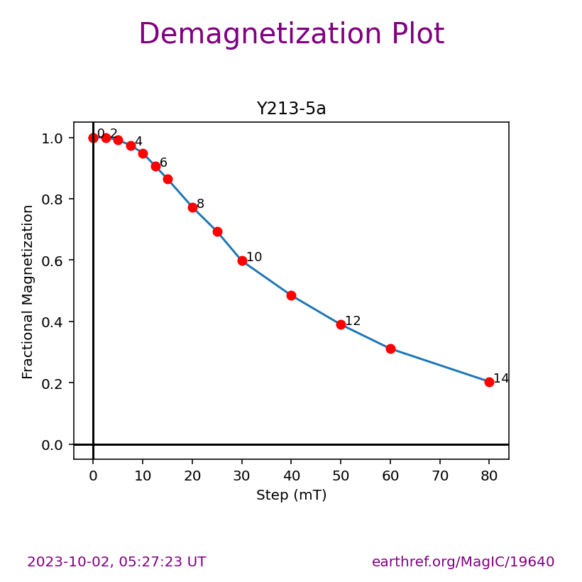
The ipmag.zeq_magic() function will plot measurement data from single specimens generating:
equal area plot
Zijderveld plot
demagnetization plot
The n_plots parameter specifies how many specimens data are generated. It will start with the first listed specimen.
ipmag.zeq_magic(save_plots=False,
                input_dir_path=directory,
                n_plots=1)
-I- Using online data model
-I- Getting method codes from earthref.org
-I- Importing controlled vocabularies from https://earthref.org
(True, [])
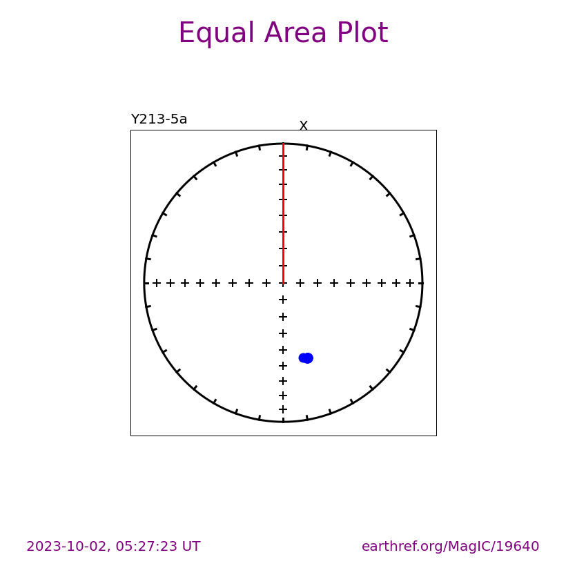
Plot a specific specimen#
We can then have ipmag.zeq_magic plot a specific specimen rather than defaulting to plotting the first one.
specimen_to_plot = 'Y217-9a'

ipmag.zeq_magic(save_plots=False,
                input_dir_path=directory,
                specimen=specimen_to_plot)
(True, [])
specimen_to_plot = 'Y213-5a'

ipmag.zeq_magic(save_plots=False,
                input_dir_path=directory,
                specimen=specimen_to_plot)
(True, [])
Visualizing site level data#
Plots can also be saved by setting save_plots to be True
ipmag.eqarea_magic(save_plots=False,
                   input_dir_path=directory,
                   dir_path=directory,
                   )
7  sites records read in
1  saved in  LO:_Mallard Lake_SI:__SA:__SP:__CO:_g_TY:_eqarea_.svg
(True, ['LO:_Mallard Lake_SI:__SA:__SP:__CO:_g_TY:_eqarea_.svg'])
ipmag.vgpmap_magic(dir_path=directory, flip=True,
                   save_plots=False,
                   lat_0=60)
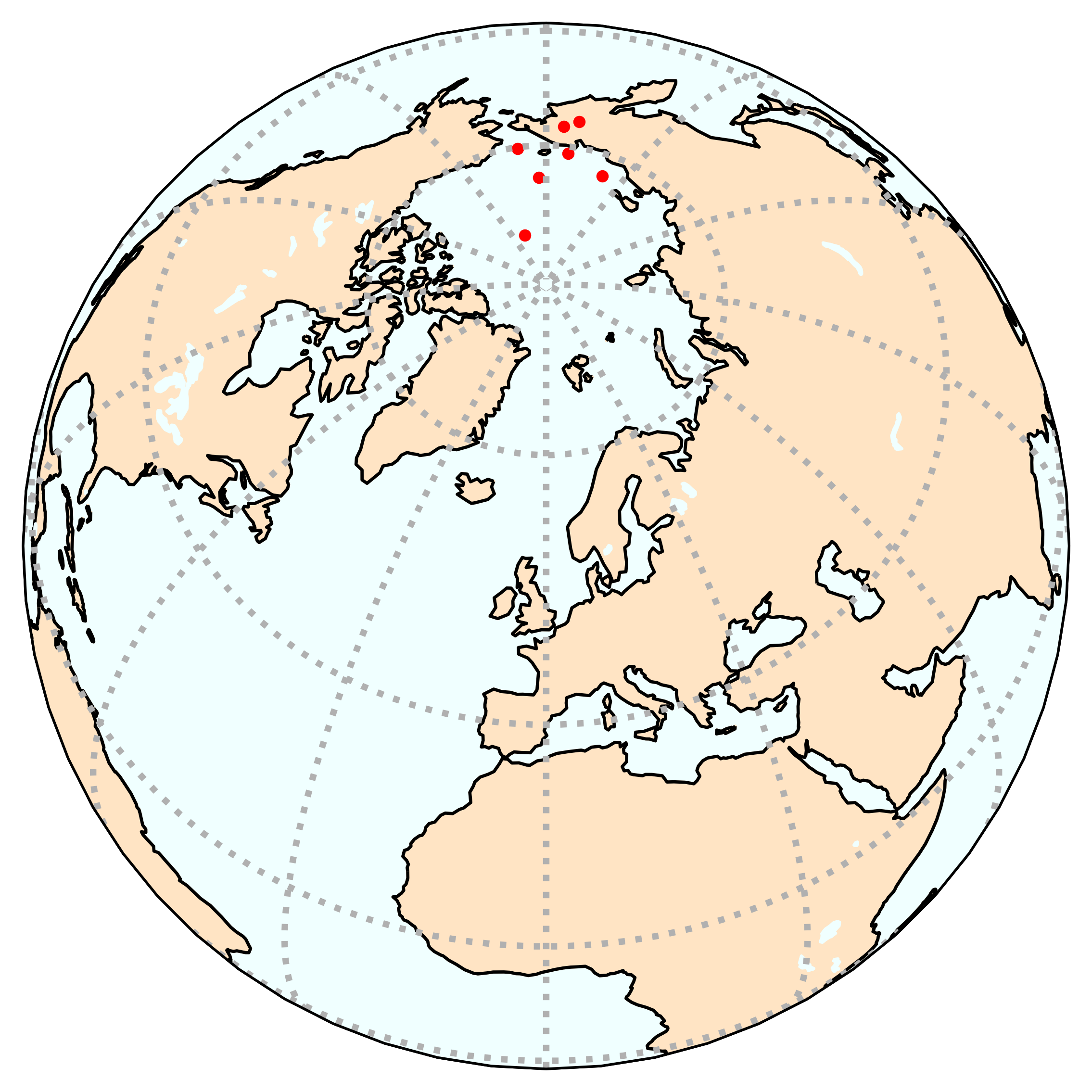
1 saved in MC:_19640_TY:_VGP_map.pdf
(True, dict_values(['MC:_19640_TY:_VGP_map.pdf']))
Importing specific MagIC tables#
The functions above ipmag.zeq_magic, ipmag.eqarea_magic, and ipmag.vgpmap_magic are convenience functions that are able to directly read from MagIC files. For some other functions in PmagPy data need to be imported to be Python objects. There is a really nice package for dealing with tabular data in Python called pandas. The code cell below imports this package so that we can use it. We use the typical scientific Python nomenclature of importing it for use to the shorthand pd.
Import the sites table#
We can now use pandas to import the sites table to a pandas dataframe using the function pd.read_csv().
sites = pd.read_csv(directory + 'sites.txt', sep='\t', header=1)
sites
| age | age_unit | analysts | citations | dir_alpha95 | dir_comp_name | dir_dec | dir_inc | dir_k | dir_n_samples | ... | method_codes | result_quality | samples | site | software_packages | specimens | vgp_dm | vgp_dp | vgp_lat | vgp_lon | |
|---|---|---|---|---|---|---|---|---|---|---|---|---|---|---|---|---|---|---|---|---|---|
| 0 | 160.2 | ka | AFP | This study | 2.4 | Y212_chrm | 352.1 | 66.2 | 396 | 8 | ... | LP-DIR-AF:DE-BFL-A:DA-DIR-GEO:LP-DIR-T:DE-BFL:... | g | Y2102-1:Y2102-2:Y2102-3:Y2102-4:Y2102-5:Y2102-... | Y2102 | pmagpy-4.2.108: demag_gui.v.3.0 | Y2102-1a:Y2102-2a:Y2102-2b:Y2102-3a:Y2102-4a:Y... | 3.9 | 3.2 | 83.1 | 199.7 |
| 1 | 159.9 | ka | AFP | This study | 7.7 | Y211_chrm | 339.3 | 66.2 | 54 | 6 | ... | LP-DIR-T:DE-BFP:DA-DIR-GEO:DE-BFL-A:LP-DIR-AF:... | g | Y211-1:Y211-2:Y211-3:Y211-4:Y211-5:Y211-7 | Y211 | pmagpy-4.2.108: demag_gui.v.3.0 | Y211-1a:Y211-2a:Y211-3a:Y211-3b:Y211-4a:Y211-5... | 12.6 | 10.3 | 75.2 | 183.1 |
| 2 | 160.2 | ka | AFP | This study | 4.9 | Y213_chrm | 332.1 | 68.1 | 87 | 1 | ... | LP-DIR-AF:DE-BFL:DA-DIR-GEO:LP-DIR-T:DE-BFL-A:... | g | Y213-10:Y213-1:Y213-2:Y213-3:Y213-4:Y213-5:Y21... | Y213 | pmagpy-4.2.108: demag_gui.v.3.0 | Y213-10a:Y213-1a:Y213-1b:Y213-2a:Y213-3a:Y213-... | 8.2 | 6.9 | 70.2 | 189.3 |
| 3 | 161.7 | ka | AFP | This study | 4.7 | Y214_chrm | 337.5 | 60.9 | 88 | 1 | ... | LP-DIR-AF:DE-BFL:DA-DIR-GEO:DE-BFL-A:LP-DIR-T:... | g | Y214-11:Y214-1:Y214-2:Y214-3:Y214-4:Y214-5:Y21... | Y214 | pmagpy-4.2.108: demag_gui.v.3.0 | Y214-11a:Y214-1a:Y214-2a:Y214-3a:Y214-4a:Y214-... | 7.2 | 5.5 | 73.5 | 157.8 |
| 4 | 160.8 | ka | AFP | This study | 3.0 | Y215_chrm | 333.3 | 64.1 | 211 | 1 | ... | LP-DIR-AF:DE-BFL:DA-DIR-GEO:DE-BFL-A:LP-DIR-T:... | g | Y215-10:Y215-1:Y215-2:Y215-3:Y215-4:Y215-5:Y21... | Y215 | pmagpy-4.2.108: demag_gui.v.3.0 | Y215-10a:Y215-1b:Y215-2a:Y215-3b:Y215-4a:Y215-... | 4.8 | 3.8 | 71.2 | 172.5 |
| 5 | 160.8 | ka | AFP | This study | 1.9 | Y216_chrm | 326.3 | 64.7 | 549 | 1 | ... | LP-DIR-T:DE-BFL:DA-DIR-GEO:LP-DIR-AF:DE-BFL-A:... | g | Y216-10:Y216-11:Y216-1:Y216-2:Y216-3:Y216-4:Y2... | Y216 | pmagpy-4.2.108: demag_gui.v.3.0 | Y216-10a:Y216-11a:Y216-1a:Y216-2a:Y216-3a:Y216... | 3.1 | 2.5 | 65.4 | 171.3 |
| 6 | 160.8 | ka | AFP | This study | 3.4 | Y217_chrm | 326.5 | 64.4 | 185 | 1 | ... | LP-DIR-AF:DE-BFL:DA-DIR-GEO:DE-BFL-A:LP-DIR-T:... | g | Y217-10:Y217-1:Y217-2:Y217-3:Y217-4:Y217-5:Y21... | Y217 | pmagpy-4.2.108: demag_gui.v.3.0 | Y217-10a:Y217-1a:Y217-2a:Y217-2b:Y217-3a:Y217-... | 5.4 | 4.4 | 66.6 | 175.1 |
7 rows × 32 columns
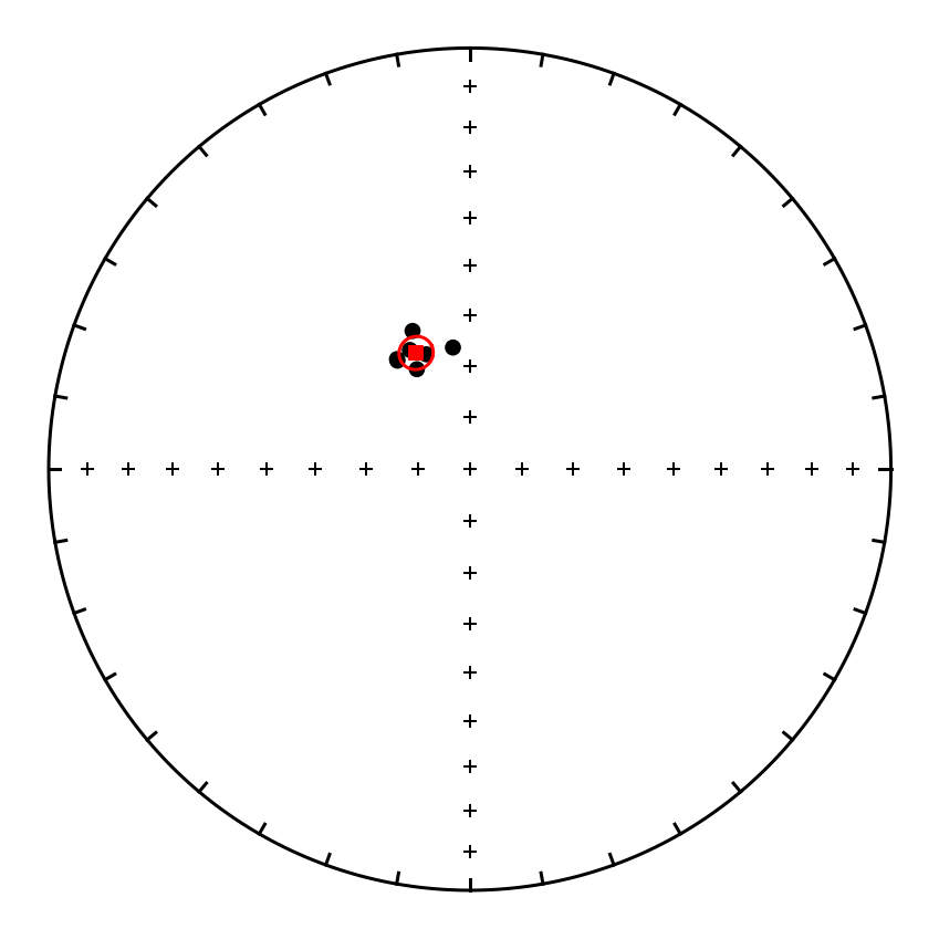
Plot the sites and calculate the Fisher mean#
We can extract specific columns from the dataframe by using the nomenclature dataframe_name['column_name']. In this case, the dataframe name is sites and the column name might be dir_dec. So sites['dir_dec'] will give us all the declinations.
sites_dec = sites['dir_dec']
sites_inc = sites['dir_inc']
plt.figure(figsize=(6,6))
ipmag.plot_net(1)
ipmag.plot_di(sites_dec, sites_inc, color='black', marker='o', markersize=40)
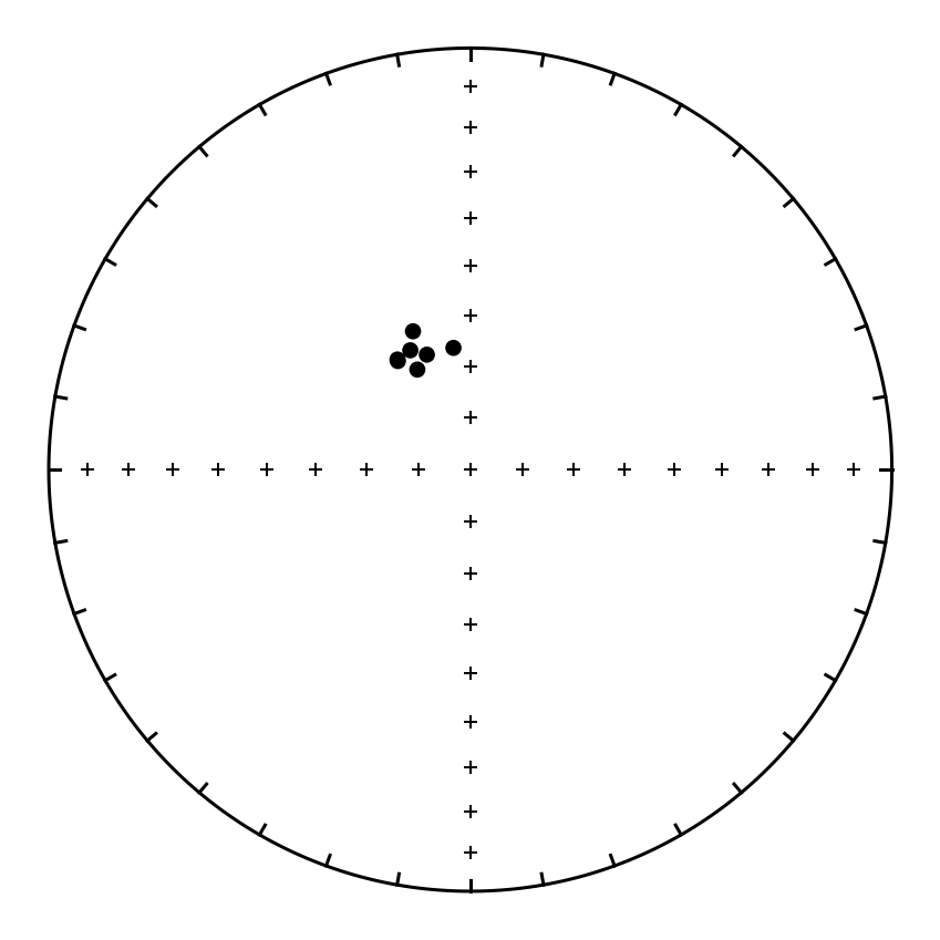
mean_direction = ipmag.fisher_mean(sites_dec, sites_inc)
ipmag.print_direction_mean(mean_direction)
Dec: 335.2  Inc: 65.2
Number of directions in mean (n): 7
Angular radius of 95% confidence (a_95): 3.2
Precision parameter (k) estimate: 348.8
plt.figure(figsize=(6,6))
ipmag.plot_net(1)
ipmag.plot_di(sites_dec, sites_inc, color='black', marker='o', markersize=40)
ipmag.plot_di_mean(mean_direction['dec'], mean_direction['inc'], mean_direction['alpha95'],
                   color='red', marker='s', markersize=40)