The Conglomerate Test#
What is a conglomerate test?#
A conglomerate test evaluates whether remanence directions measured from individual clasts in a conglomerate or diamictite are statistically consistent with a random distribution. The logic is that if the clasts acquired their magnetization before erosion, transport, and deposition, then subsequent physical reorientation during deposition should disperse their directions. Graham (1949) introduced this field test as a way to assess the relative timing of magnetization acquisition in sedimentary settings.
If the clast magnetization directions are consistent with randomness, then:
The magnetization was likely acquired before the conglomerate formed.
This constitutes a positive conglomerate test.
If the clast directions are significantly clustered rather than random, then:
The magnetization was likely acquired after conglomerate formation, for example during a later thermal or chemical remagnetization event.
This constitutes a negative conglomerate test.
A positive conglomerate test is one of the strongest field tests for supporting the primary nature of a magnetization, because the clast reorientation occurred during deposition of the conglomerate or diamictite. That makes the test especially valuable for establishing that a remanence predates lithification and later tectonic or diagenetic events.
Statistical framework: Watson’s \(R_o\) test#
Watson (1956) formalized a test for whether a set of directions is consistent with randomness on the sphere using the resultant vector length \(R\). Given \(n\) unit vectors, the resultant vector \(\mathbf{R}\) is their vector sum, and its length \(R\) ranges from 0 for a highly dispersed population to \(n\) for perfectly aligned directions:
The null hypothesis is that the directions are drawn from a uniform random distribution on the sphere. Watson (1956) derived critical values \(R_o\) such that the probability of obtaining \(R \geq R_o\) from a random distribution is less than 5% or 1%. These critical values depend only on \(n\). For small sample sizes, tabulated values should be used; for larger sample sizes, a chi-square approximation is commonly used.
A commonly used approximation is:
\(R_{o,95} = \sqrt{7.815 \cdot n / 3}\)
\(R_{o,99} = \sqrt{11.345 \cdot n / 3}\)
The decision rule is:
If \(R < R_{o,95}\): the null hypothesis of randomness cannot be rejected \(\rightarrow\) the test passes
If \(R > R_{o,95}\): the null hypothesis of randomness is rejected \(\rightarrow\) the test fails
Application#
In this notebook, we apply the conglomerate test to data from the Cryogenian Ayn Formation of Oman from the following study for which there are data in the MagIC database:
Swanson-Hysell, N. L., Zhang, Y., Macdonald, F. A., Koran, I., Tasistro-Hart, A. R., and Jay, A. F. (2025). Oman was on the northern margin of a wide late Tonian Mozambique Ocean. Geology. doi:10.1130/G53450.1
Multiple magnetization components were isolated from clasts within this diamictite. A component acquired before conglomerate formation should show random directions (passing the test), while a post-depositional overprint should show coherent directions (failing the test).
References#
Graham, J. W. (1949). The stability and significance of magnetism in sedimentary rocks. J. Geophys. Res., 54, 131–167.
Watson, G. S. (1956). A test for randomness of directions. Mon. Not. R. Astron. Soc. Geophys. Suppl., 7, 160–161.
Import packages#
import pmagpy.ipmag as ipmag
import pmagpy.pmag as pmag
import pandas as pd
import numpy as np
import matplotlib.pyplot as plt

%matplotlib inline
%config InlineBackend.figure_format='retina'
Download and unpack data from MagIC#
directory = './data/SwansonHysell2025'
result, magic_file_path = ipmag.download_magic_from_id('20340', directory=directory)
ipmag.unpack_magic(magic_file_path, dir_path=directory, print_progress=False)
Download successful. File saved to: ./data/SwansonHysell2025/magic_contribution_20340.txt
1  records written to file  /Users/hematite/Documents/GitHub/PmagPy-docs/example_notebooks/template_notebooks/data/SwansonHysell2025/contribution.txt
1  records written to file  /Users/hematite/Documents/GitHub/PmagPy-docs/example_notebooks/template_notebooks/data/SwansonHysell2025/locations.txt
207  records written to file  /Users/hematite/Documents/GitHub/PmagPy-docs/example_notebooks/template_notebooks/data/SwansonHysell2025/sites.txt
386  records written to file  /Users/hematite/Documents/GitHub/PmagPy-docs/example_notebooks/template_notebooks/data/SwansonHysell2025/samples.txt
1454  records written to file  /Users/hematite/Documents/GitHub/PmagPy-docs/example_notebooks/template_notebooks/data/SwansonHysell2025/specimens.txt
29425  records written to file  /Users/hematite/Documents/GitHub/PmagPy-docs/example_notebooks/template_notebooks/data/SwansonHysell2025/measurements.txt
True
Load data for the AynC conglomerate site#
The AynC site is a diamictite from the Ayn Formation in which individual clasts were sampled and demagnetized. The sites table provides site-level Fisher statistics (including \(R\) and \(n\)) for each magnetization component. The specimens table provides the individual clast directions that we can plot on stereonets.
Two magnetization components are of interest:
lt (low temperature): removed at low demagnetization temperatures — typically a viscous or chemical overprint acquired after deposition
mag (magnetite): the characteristic remanence carried by magnetite — this represents the primary magnetization of the clasts’ source rocks
sites = pd.read_csv(directory + '/sites.txt', sep='\t', header=1)

# filter for AynC site with directional data
aync_sites = sites[(sites.site == 'AynC') & sites.dir_dec.notna()].copy()
aync_sites[['site', 'dir_comp_name', 'dir_dec', 'dir_inc', 'dir_alpha95',
            'dir_r', 'dir_k', 'dir_n_samples']]
| site | dir_comp_name | dir_dec | dir_inc | dir_alpha95 | dir_r | dir_k | dir_n_samples | |
|---|---|---|---|---|---|---|---|---|
| 0 | AynC | lt | 8.0 | 27.3 | 6.4 | 15.5562 | 34.0 | 16.0 |
| 1 | AynC | mag | 315.5 | 41.3 | 71.8 | 3.8924 | 1.0 | 16.0 |
| 2 | AynC | mt | 64.1 | 46.7 | 39.3 | 6.0077 | 3.0 | 9.0 |
Plot clast directions by component#
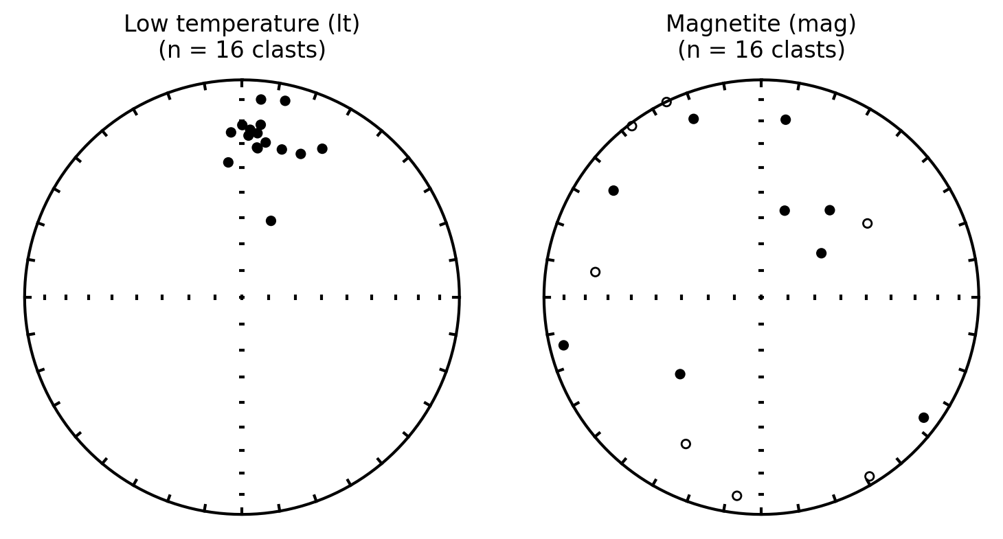
We read the specimen-level directions for the AynC clasts in geographic coordinates (dir_tilt_correction == 0) and plot each component on an equal area stereonet. Visually, random directions should fill the stereonet, while a coherent overprint will cluster.
specimens = pd.read_csv(directory + '/specimens.txt', sep='\t', header=1)

# filter for AynC specimens in geographic coordinates
aync_spec = specimens[(specimens.specimen.str.startswith('AynC')) &
                      (specimens.dir_dec.notna()) &
                      (specimens.dir_tilt_correction == 0)].copy()

components = ['lt', 'mag']
titles = ['Low temperature (lt)', 'Magnetite (mag)']

fig, axes = plt.subplots(1, 2, figsize=(9, 4))
for ax, comp, title in zip(axes, components, titles):
    plt.sca(ax)
    ipmag.plot_net()
    comp_data = aync_spec[aync_spec.dir_comp == comp]
    ipmag.plot_di(comp_data.dir_dec.tolist(), comp_data.dir_inc.tolist())
    plt.title(f'{title}\n(n = {len(comp_data)} clasts)')
plt.tight_layout()
plt.show()
Apply Watson’s conglomerate test#
We now apply the Watson (1956) test to each component using the site-level \(R\) and \(n\) values from the sites table. The function ipmag.conglomerate_test_Watson() compares the observed \(R\) to the critical \(R_o\) values.
We expect:
The lt component (low-temperature overprint) to fail — its directions should be coherent because the overprint was acquired after the conglomerate formed.
The mag component (primary magnetite remanence) to pass — its directions should be random because the magnetization predates clast deposition.
Low temperature (lt) component#
lt = aync_sites[aync_sites.dir_comp_name == 'lt'].iloc[0]
ipmag.conglomerate_test_Watson(lt.dir_r, int(lt.dir_n_samples))
R = 15.5562
Ro_95 = 6.4
Ro_99 = 7.6
The null hypothesis of randomness can be rejected at the 95% confidence level
The null hypothesis of randomness can be rejected at the 99% confidence level
{'n': 16, 'R': np.float64(15.5562), 'Ro_95': 6.4, 'Ro_99': 7.6}
Magnetite (mag) component#
mag = aync_sites[aync_sites.dir_comp_name == 'mag'].iloc[0]
ipmag.conglomerate_test_Watson(mag.dir_r, int(mag.dir_n_samples))
R = 3.8924
Ro_95 = 6.4
Ro_99 = 7.6
This population "passes" a conglomerate test as the null hypothesis of randomness cannot be rejected at the 95% confidence level
{'n': 16, 'R': np.float64(3.8924), 'Ro_95': 6.4, 'Ro_99': 7.6}
Interpretation#
The results illustrate the power of the conglomerate test for distinguishing primary and secondary magnetizations:
The lt component has a large \(R\) relative to \(R_o\) — the clast directions are not random. This low-temperature component was acquired after conglomerate deposition, as can also be seen from the similarity between this component’s direction and the present local field direction (Fig. 2 in Swanson-Hysell et al., 2025). The test fails.
The mag component has \(R\) of 3.9 which is well below \(R_{o,95}\) of 6.4 — the clast directions are indistinguishable from random. This indicates pre-depositional magnetization: the magnetite remanence in the fine-grained mafic clasts (likely sourced from the Shaat dikes) was acquired before the clasts were incorporated into the Cryogenian Ayn Formation diamictite. The test passes.
Swanson-Hysell et al. (2025) wrote: “Well-resolved magnetite magnetization is constrained to be primary by a conglomerate test on mafic clasts within overlying Cryogenian diamictite.” This positive conglomerate test supports the interpretation that the ca. 726 Ma Shaat dike paleomagnetic pole can be used to reconstruct Oman’s late Tonian paleogeography.