In this notebook, a contribution is downloaded from the MagIC database. Susceptibility-temperature (-T) data contained within it are extracted. The user has the option to correct for the diamagnetic signal of the measurement instrument and holder (optional) and to smooth the data prior to further analysis (optional).
The notebook is to be run cell-by-cell to allow users to select corrections/filters as needed. The code below brings in example magnetite data from the rock magnetic bestiary. Any MagIC contribution that contains -T data can be used in place of this example dataset.
This notebook focuses on importing, correcting, and plotting -T data; quantitative Curie temperature estimation is demonstrated in the companion Curie temperature estimation notebook.
Install and import packages
import pmagpy.rockmag as rmag
import pmagpy.ipmag as ipmag
import pmagpy.contribution_builder as cb

from bokeh.io import output_notebook
output_notebook(hide_banner=True)Import data
We follow one of the approaches as in the rockmag_data_unpack.ipynb notebook to bring the MagIC data into the notebook as a Contribution.
#define these three parameters to match your data
magic_id = '20354'
share_key = '2f33e164-df55-4548-8d28-5b715683ae43'
dir_path = 'example_data/X-T'

result, magic_file = ipmag.download_magic_from_id(magic_id, directory=dir_path, share_key=share_key)
ipmag.unpack_magic(magic_file, dir_path, print_progress=False)
contribution = cb.Contribution(dir_path)
measurements = contribution.tables['measurements'].df
Download successful. File saved to: example_data/X-T/magic_contribution_20354.txt
1 records written to file /Users/penokean/0000_GitHub/RockmagPy-notebooks/thermomagnetic_notebooks/example_data/X-T/contribution.txt
2 records written to file /Users/penokean/0000_GitHub/RockmagPy-notebooks/thermomagnetic_notebooks/example_data/X-T/locations.txt
2 records written to file /Users/penokean/0000_GitHub/RockmagPy-notebooks/thermomagnetic_notebooks/example_data/X-T/sites.txt
43 records written to file /Users/penokean/0000_GitHub/RockmagPy-notebooks/thermomagnetic_notebooks/example_data/X-T/samples.txt
201 records written to file /Users/penokean/0000_GitHub/RockmagPy-notebooks/thermomagnetic_notebooks/example_data/X-T/specimens.txt
92035 records written to file /Users/penokean/0000_GitHub/RockmagPy-notebooks/thermomagnetic_notebooks/example_data/X-T/measurements.txt
-I- Using online data model
-I- Getting method codes from earthref.org
-I- Importing controlled vocabularies from https://earthref.org
The project export contains data from all the experiments
Each measurement in a MagIC measurements table has a method_codes value. These method codes come from a “controlled vocabulary” (https://
In the method codes used for the example contribution:
LPrefers to lab protocolX-Trefers to susceptibility vs. temperature experiments done on the Kappabridge
measurements = measurements[measurements['method_codes'].str.contains('LP-X-T', na=False)]Select a -T experiment
Creates a dropdown to select specimens with -T data.
specimen, experiment = rmag.specimen_experiment_selection_interactive(measurements)Plot -T data
If the remove_holder parameter is set to be True, we assume that the lowest susceptibility value during the whole measurement is the holder signal. This assumption relies on this value being after the specimen is heated above the critical temperature such that it is paramagnetic and the holder signal is dominant.
selected_experiment = measurements[(measurements['specimen']==specimen.value) &
                                      (measurements['experiment']==experiment.value)].reset_index(drop=True)

rmag.plot_chi_T(selected_experiment,
              temp_unit='C',
              remove_holder=True,
              plot_derivative=False,
plot_inverse=False)Plot -T data with derivative
In this example, the experiment 'IRM-KappaF-LP-X-T-3410' is selected by name (rather than with the dropdown above) and is plotted together with its derivative by setting plot_derivative=True.
selected_experiment = rmag.experiment_selection(measurements, 'IRM-KappaF-LP-X-T-3410')

rmag.plot_chi_T(selected_experiment,
              temp_unit='C',
              remove_holder=True,
              plot_derivative=True,
plot_inverse=False)Inverse susceptibility
Above its Curie temperature (Tc) a mineral phase is paramagnetic, so the inverse susceptibility 1/ has a linear positive slope above Tc (Petrovský and Kapička, 2006). Setting plot_inverse=True in rmag.plot_chi_T() adds the 1/ panel for visual inspection of where Curie–Weiss (paramagnetic) behavior sets in.
Quantitative Curie temperature estimation from these data — inflection point, maximum curvature, two-tangent, inverse susceptibility (Curie–Weiss), and Landau fitting, with their physical basis and caveats — is demonstrated in the companion Curie temperature estimation notebook.
rmag.plot_chi_T(selected_experiment,
              temp_unit='C',
              remove_holder=True,
              plot_derivative=True,
plot_inverse=True,)Appendix: determining the best temperature window for smoothing
Smoothing of -T data prior to analysis is optional and is applied through the smooth_window parameter of rmag.plot_chi_T() (a running average with the given temperature window; the default of smooth_window=0 applies no smoothing). Rather than picking a window size arbitrarily, the window size can be chosen based on the trade-off between smoothness and misfit.
The rmag.optimize_moving_average_window() function plots the model roughness against the root mean square error of the model (note that the y-axis is inverted) (a measure of the difference between the running average and the data). Each point on the graph is for a different temperature window size. The knee in the curve (the break of slope) can be interpreted as the optimal temperature window for smoothing. At this point (window) there is a decent trade off between the smoothness of the model (the running average) and error on the model.
Set values for min_temp_window and max_temp_window to set the temperature range for exploring the rms and variance tradeoff.
min_temp_window = 0
max_temp_window = 50
steps = 20
fig, ax = rmag.optimize_moving_average_window(selected_experiment, min_temp_window, max_temp_window, steps=steps)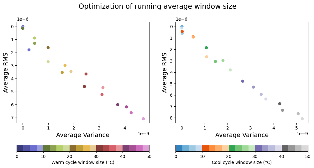
Upon inspecting the plot, a smoothing window size of about 10 K seems to be a good choice for this dataset. The chosen window can then be applied by passing it to the smooth_window parameter of rmag.plot_chi_T():
rmag.plot_chi_T(selected_experiment,
              temp_unit='C',
              remove_holder=True,
              plot_derivative=True,
smooth_window=10)References
Petrovský, E., & Kapička, A. (2006). On determination of the Curie point from thermomagnetic curves. Journal of Geophysical Research: Solid Earth, 111, B12S27. Petrovský & Kapička (2006)
Additional references for the Curie temperature estimation methods are given in the companion Curie temperature estimation notebook.
- Petrovský, E., & Kapička, A. (2006). On determination of the Curie point from thermomagnetic curves. Journal of Geophysical Research: Solid Earth, 111, B12S27. 10.1029/2006JB004507