The Curie temperature (T) is the temperature at which a ferromagnetic (sensu lato) mineral undergoes the transition to a paramagnetic state. Because T varies systematically with composition within solid-solution series such as the titanomagnetites, it is one of the most diagnostic rock magnetic parameters for magnetic mineralogy. However, estimates of T from thermomagnetic data are method-dependent and data-type-dependent, with systematic offsets of several to tens of degrees between methods applied to the same curve (Lattard et al., 2006; Fabian et al., 2013). This notebook demonstrates the estimation methods implemented in rockmag.py, their physical basis, and the caveats that attend each of them.
Method overview
The analysis of Fabian et al. (2013), grounded in the Landau theory of second-order phase transitions with an explicit field term, provides the framework. For a magnetization curve M(T) measured in an applied field, the Curie temperature corresponds to the inflection point of the curve (the minimum of dM/dT), a position that is effectively independent of the applied field. The classical estimators — the maximum curvature method (“the temperature at which the curvature of the concave part of the heating curve is a maximum”; Ade-Hall et al., 1965) and the two-tangent method of Grommé et al. (1969) — coincide with each other and lie systematically above the inflection-point T, typically by 10–15 °C, with the offset increasing with field strength.
Low-field susceptibility (T) requires separate treatment. At least four physical processes contribute to the initial susceptibility near the ordering temperature (variation of M with field, rotation against anisotropy, domain-wall motion, and superparamagnetism), so the shape of (T) near T is strongly grain-size dependent, and a Hopkinson peak marks the blocking temperature rather than T. For (T) data, Petrovský and Kapička (2006) showed that the two-tangent method lacks a rigorous physical basis and can considerably overestimate T; they advocate the inverse susceptibility approach, in which 1/ above the transition is extrapolated to zero via the Curie-Weiss law — with the caveat that this yields the paramagnetic Curie temperature T.
| method | intended data | what it locates | key caveat |
|---|---|---|---|
inflection | in-field M(T) | T (Landau theory) | requires smoothing; derivatives amplify noise |
max_curvature | M(T) | practical T of Ade-Hall et al. (1965) | above inflection-point T by ~10–15 °C; field-dependent |
two_tangent | M(T) | graphical “knee” (Grommé et al., 1969) | coincides with max curvature; lacks a rigorous basis on (T) |
inverse_susceptibility | (T) | paramagnetic Curie temperature | T; sensitive to the fitting window |
landau | in-field M(T) | T with formal uncertainty (Fabian et al., 2013) | single phase measured through its transition |
ms_squared_extrapolation | M(T) that ends below T | T by extrapolating M 0 (Moskowitz, 1981) | reliability decays with distance below T; highest-T phase only |
All of these are available through individual functions (rmag.curie_derivative_estimates, rmag.curie_two_tangent, rmag.curie_inverse_susceptibility, rmag.curie_landau_fit, rmag.curie_Ms_squared_extrapolation) that operate on plain temperature/magnetization arrays, and through the wrapper rmag.curie_temperature_estimates that takes a MagIC-formatted experiment DataFrame and returns a tidy comparison table.
Install and import packages
import numpy as np
import pandas as pd
import matplotlib.pyplot as plt

import pmagpy.rockmag as rmag
import pmagpy.ipmag as ipmag
import pmagpy.contribution_builder as cb

from bokeh.io import output_notebook
output_notebook(hide_banner=True)Import data
The examples in this notebook use data from the Rock Magnetic Bestiary contribution to the MagIC database that includes measurements on synthetic magnetite, titanomagnetite, and maghemite samples. We follow the approach of the rockmag_data_unpack.ipynb notebook to bring the MagIC data into the notebook as a contribution.
The rmag.make_experiment_df helper tabulates the unique specimen/method/experiment combinations in the measurements table; inspecting it (or using the selection widgets shown in the companion notebooks) is how the experiment names used by name below can be found.
# define these three parameters to match your data
# (the download goes to a folder unique to this notebook so that other
# notebooks unpacking contributions into a shared folder cannot overwrite
# the tables used here)
magic_id = '20354'
share_key = '2f33e164-df55-4548-8d28-5b715683ae43'
dir_path = 'example_data/curie_X-T'

result, magic_file = ipmag.download_magic_from_id(magic_id, directory=dir_path, share_key=share_key)
ipmag.unpack_magic(magic_file, dir_path, print_progress=False)
contribution = cb.Contribution(dir_path)
measurements = contribution.tables['measurements'].df
experiments = rmag.make_experiment_df(measurements)
Download successful. File saved to: example_data/curie_X-T/magic_contribution_20354.txt
1 records written to file /Users/penokean/0000_GitHub/RockmagPy-notebooks/thermomagnetic_notebooks/example_data/curie_X-T/contribution.txt
2 records written to file /Users/penokean/0000_GitHub/RockmagPy-notebooks/thermomagnetic_notebooks/example_data/curie_X-T/locations.txt
2 records written to file /Users/penokean/0000_GitHub/RockmagPy-notebooks/thermomagnetic_notebooks/example_data/curie_X-T/sites.txt
43 records written to file /Users/penokean/0000_GitHub/RockmagPy-notebooks/thermomagnetic_notebooks/example_data/curie_X-T/samples.txt
201 records written to file /Users/penokean/0000_GitHub/RockmagPy-notebooks/thermomagnetic_notebooks/example_data/curie_X-T/specimens.txt
92035 records written to file /Users/penokean/0000_GitHub/RockmagPy-notebooks/thermomagnetic_notebooks/example_data/curie_X-T/measurements.txt
-I- Using online data model
-I- Getting method codes from earthref.org
-I- Importing controlled vocabularies from https://earthref.org
Part 1: Curie temperature from magnetization M(T) data
Strong-field thermomagnetic curves — from a Curie balance or a vibrating sample magnetometer (VSM) — measure the induced magnetization through the transition and are the preferred data type for quantitative T estimation. The per-method estimator functions operate on plain arrays, so data from any acquisition stream can be analyzed. Here we use a classic Curie balance heating curve that has long shipped with PmagPy as curie_example.dat (a plain two-column temperature/magnetization file), which allows direct comparison with the legacy ipmag.curie function.
Each estimator returns a dictionary with the estimate itself (curie_temp, plus curie_temp_stderr where the method provides a formal uncertainty), a params dictionary of fit parameters, and a diagnostics dictionary of arrays (derivatives, fitted lines, model curves) for plotting — used to build the figure below. The derivative estimator instead names its two estimates inflection_temp and max_curvature_temp.
T, M = np.loadtxt('../example_data/curie/curie_example.dat', unpack=True)

# smooth with a 10 degree moving window prior to differentiation
sT, sM = rmag.smooth_moving_average(T, M, 10)

derivative_result = rmag.curie_derivative_estimates(sT, sM, smooth_window=10)
two_tangent_result = rmag.curie_two_tangent(sT, sM)
landau_result = rmag.curie_landau_fit(sT, sM, temp_unit='C')

print(f"inflection point:      {derivative_result['inflection_temp']:.1f} °C")
print(f"maximum curvature:     {derivative_result['max_curvature_temp']:.1f} °C")
print(f"two-tangent:           {two_tangent_result['curie_temp']:.1f} °C")
print(f"Landau fit:            {landau_result['curie_temp']:.1f} ± {landau_result['curie_temp_stderr']:.1f} °C  (h = {landau_result['params']['h']:.2e})")
inflection point: 480.3 °C
maximum curvature: 548.2 °C
two-tangent: 541.2 °C
Landau fit: 547.8 ± 2.4 °C (h = 1.56e-04)
fig, (ax1, ax2) = plt.subplots(2, 1, figsize=(9, 8), sharex=True)

ax1.scatter(T, M, s=6, color='#bbbbbb', label='measured')
ax1.plot(sT, sM, color='#333333', lw=1.5, label='smoothed (10 °C window)')
ax1.plot(landau_result['diagnostics']['model_T'], landau_result['diagnostics']['model_M'],
         color='#CC79A7', lw=1.5, label='Landau model fit')
for temp, label, color in [
        (derivative_result['inflection_temp'], 'inflection', '#0072B2'),
        (derivative_result['max_curvature_temp'], 'max curvature', '#E69F00'),
        (two_tangent_result['curie_temp'], 'two-tangent', '#009E73'),
        (landau_result['curie_temp'], 'Landau fit', '#CC79A7')]:
    ax1.axvline(temp, color=color, lw=1.2, label=f'{label}: {temp:.0f} °C')
ax1.set_ylabel('M (arbitrary units)')
ax1.legend(fontsize=9)

d = derivative_result['diagnostics']
ax2.plot(d['T'], d['dy_dT'], color='#333333', lw=1.2)
ax2.axvline(derivative_result['inflection_temp'], color='#0072B2', lw=1.2)
ax2.set_xlabel('Temperature (°C)')
ax2.set_ylabel('dM/dT')
for ax in (ax1, ax2):
    ax.grid(alpha=0.4)
plt.tight_layout();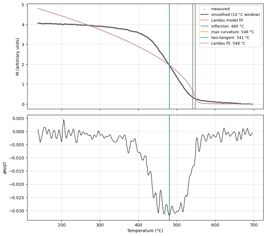
Interpreting the spread of estimates
The estimates span nearly 70 °C, and the spread itself is informative. The two-tangent (~541 °C), Landau-fit (~548 °C), and maximum-curvature (~548 °C) estimates cluster near the “knee” of the curve, while the inflection point (minimum of dM/dT, ~480 °C) sits well below it. For an ideal single-phase sample the estimates would differ by only 10–15 °C, with the inflection point lowest and the maximum-curvature and two-tangent estimates approximately coincident above it. The much larger spread here is consistent with a distribution of Curie temperatures in this natural sample (e.g., variable titanium substitution): a T distribution broadens and flattens the steepest-descent region of the aggregate curve, so the inflection sits well below the knee — where the last ferromagnetic contribution vanishes and which traces the upper end of the distribution (Fabian et al., 2013). Comparing methods therefore provides a diagnostic of sample homogeneity that no single estimate conveys.
The reduced field h printed with the Landau fit is the model’s dimensionless applied-field parameter: it rounds the transition and generates the field-induced magnetization tail that persists above T, which is why the fit needs no ad-hoc baseline subtraction.
Because differentiation amplifies noise, the first and second derivatives are smoothed on the same 10 °C scale as the signal (the smooth_window argument) before their extrema are located, so the inflection is placed at the center of the broad steepest-descent region rather than at an arbitrary point-to-point noise spike within it. Note the distinction between the two uses of the 10 °C window in the code above: smooth_moving_average smooths the signal once, while smooth_window=10 inside curie_derivative_estimates smooths the derivatives computed from it.
For reference, the legacy ipmag.curie function (second-derivative maximum after Bartlett smoothing on a resampled 1 °C grid) yields 552 °C on this file with the same window — consistent with the max_curvature estimate here (~548 °C), which supersedes it.
When the run ends below T: M extrapolation
Some samples cannot be measured through their transition — the classic case being titanomaghemites that chemically invert upon heating before M reaches zero. For such curves, Moskowitz (1981) proposed extrapolating on the basis that near T, mean-field theory gives M (T T), so M is linear in temperature and extrapolates to zero at T. The curie_Ms_squared_extrapolation function implements this.
To illustrate both the method and its central caveat, we truncate the example curve at 500 °C — as if the measurement had ended there — and extrapolate from the descending limb:
truncated = sT <= 500
ms2_result = rmag.curie_Ms_squared_extrapolation(sT[truncated], sM[truncated],
                                                 fit_range=(430, 500))
print(f"Ms^2 extrapolation (truncated at 500 °C): "
      f"{ms2_result['curie_temp']:.1f} ± {ms2_result['curie_temp_stderr']:.1f} °C "
      f"(r^2 = {ms2_result['params']['r_squared']:.3f})")
Ms^2 extrapolation (truncated at 500 °C): 510.3 ± 0.4 °C (r^2 = 0.996)
The fit is excellent statistically (r 0.996) yet the extrapolated T of ~510 °C falls well short of the ~548 °C obtained from the full curve — precisely because this sample has a distribution of Curie temperatures, so the descending limb available below 500 °C is not the mean-field tail of the highest-T phase. This is the caveat to carry: the extrapolation is exact for an ideal mean-field single phase (Moskowitz reported ±5 °C on FeO, Ni, and CrO standards), but its reliability decays with the distance between the last measured point and T, a goodness-of-fit statistic does not capture that model error, and for multiphase samples only the highest-T phase is (at best) recovered. Report the fitting window with the estimate, and prefer through-transition data whenever the sample allows it.
Part 2: Curie temperature from susceptibility (T) data
High-temperature susceptibility (χ-T) curves measured on a Kappabridge pass fully through the transition and are the most common thermomagnetic data type. As laid out in the method overview, the shape of (T) near T convolves several susceptibility mechanisms, so estimates from (T) require more care than those from M(T). Here we analyze the χ-T curve for a synthetic magnetite (Wright Company sample 112982) from the Rock Magnetic Bestiary.
Choosing a smoothing window
Derivative-based estimators amplify measurement noise, so the data are smoothed with a temperature-space moving window prior to differentiation. The choice of window width trades noise reduction against distortion of the curve; rmag.optimize_moving_average_window sweeps window widths and plots the residual roughness (average RMS) against the within-window variance so that a window at the “knee” of the trade-off can be chosen. For these data a ~10 °C window is a reasonable choice.
selected_experiment = measurements[measurements['experiment'] ==
                                   'IRM-KappaF-LP-X-T-3410'].reset_index(drop=True)

fig, axs = rmag.optimize_moving_average_window(selected_experiment, min_temp_window=0,
                                               max_temp_window=50, steps=20)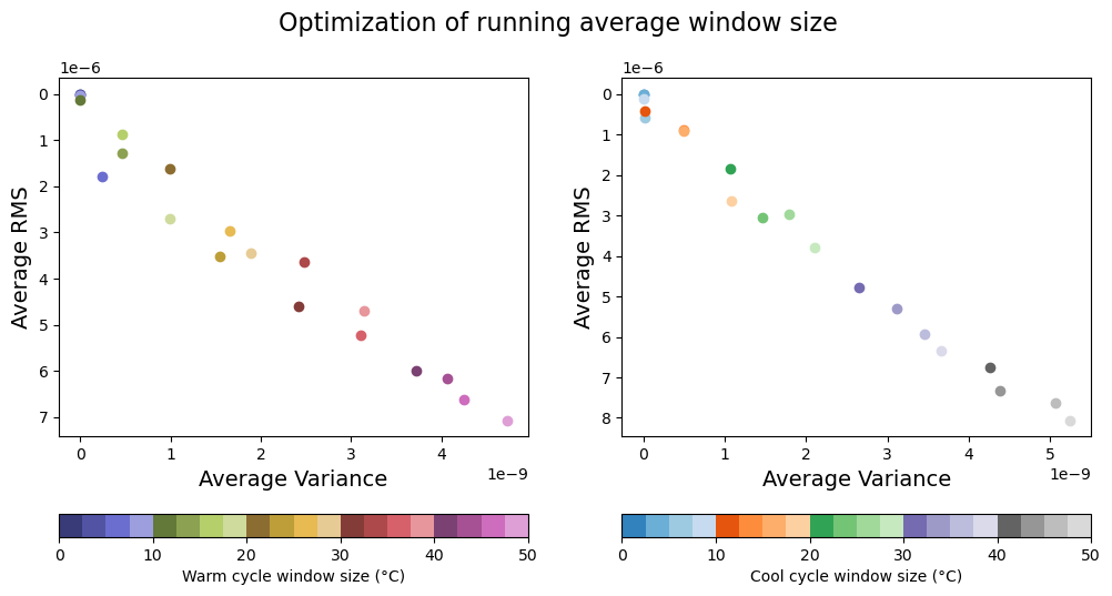
Choosing the Curie-Weiss fitting window: resolution matters
The Curie-Weiss fit must be restricted to temperatures where the signal is fully paramagnetic and still resolved by the instrument. Above the transition the holder-corrected susceptibility of this specimen collapses rapidly toward the measurement resolution of the Kappabridge: by ~625 °C the signal is pinned at the last one or two counts of the meter, producing flat quantized plateaus in 1/. Including such resolution-limited points flattens the fitted slope and biases low. A naive wide window demonstrates the failure — and the function detects it:
heating = rmag.prepare_thermomag_branches(selected_experiment, smooth_window=10)['heating']

naive_fit = rmag.curie_inverse_susceptibility(heating['T'], heating['y'], fit_range=(600, 700))
print(f"theta (600-700 °C window): {naive_fit['curie_temp']:.1f} ± {naive_fit['curie_temp_stderr']:.1f} °C")
print(f"warning: {naive_fit['params']['warning']}")
theta (600-700 °C window): 564.6 ± 9.3 °C
warning: 92% of the fitted points repeat identical susceptibility values (weak, resolution-limited signal); theta is likely biased low — tighten fit_range or set min_chi
The naive window returns 565 °C — below the inflection-point estimate of the Curie temperature. Since theory requires T, a Curie-Weiss that falls below an independent T estimate is itself a red flag that the fit is contaminated. Restricting the window to the interval where 1/ is linear and the signal remains resolved above the quantization floor recovers a fit that is both statistically better and physically consistent. Here that interval is 585–606 °C, identified by inspecting where 1/ is linear before the quantized plateaus begin — the interactive fitting tool demonstrated below is designed for exactly this. (Alternatively, the min_chi argument of curie_inverse_susceptibility screens out points below a susceptibility floor, such as a few instrument counts.)
Estimates from all methods, with the comparison table
rmag.curie_temperature_estimates applies the requested methods to the heating and cooling branches and returns a tidy DataFrame. The default method set depends on the data type, which is inferred from the magnetic_column name (columns containing susc or chi are treated as susceptibility; pass data_type to override): susceptibility data default to inflection, max_curvature, and inverse_susceptibility, while magnetization data default to inflection, max_curvature, two_tangent, and landau.
Per-method options are passed through method_kwargs, a dictionary keyed by method name whose values are keyword arguments forwarded to that method’s function — for example {'inverse_susceptibility': {'fit_range': (585, 606)}} below, or {'landau': {'fit_range': (300, 650)}}. The Curie-Weiss fit window is set explicitly — the window is part of the analysis and should be reported alongside the estimate.
curie_estimates = rmag.curie_temperature_estimates(
    selected_experiment,
    smooth_window=10,
    method_kwargs={'inverse_susceptibility': {'fit_range': (585, 606)}},
)
curie_estimates[['branch', 'method', 'curie_temp', 'curie_temp_stderr', 'temp_unit', 'notes']]rmag.plot_curie_estimates(
selected_experiment,
smooth_window=10,
method_kwargs={'inverse_susceptibility': {'fit_range': (586, 604)}},
figsize=(10, 10),
);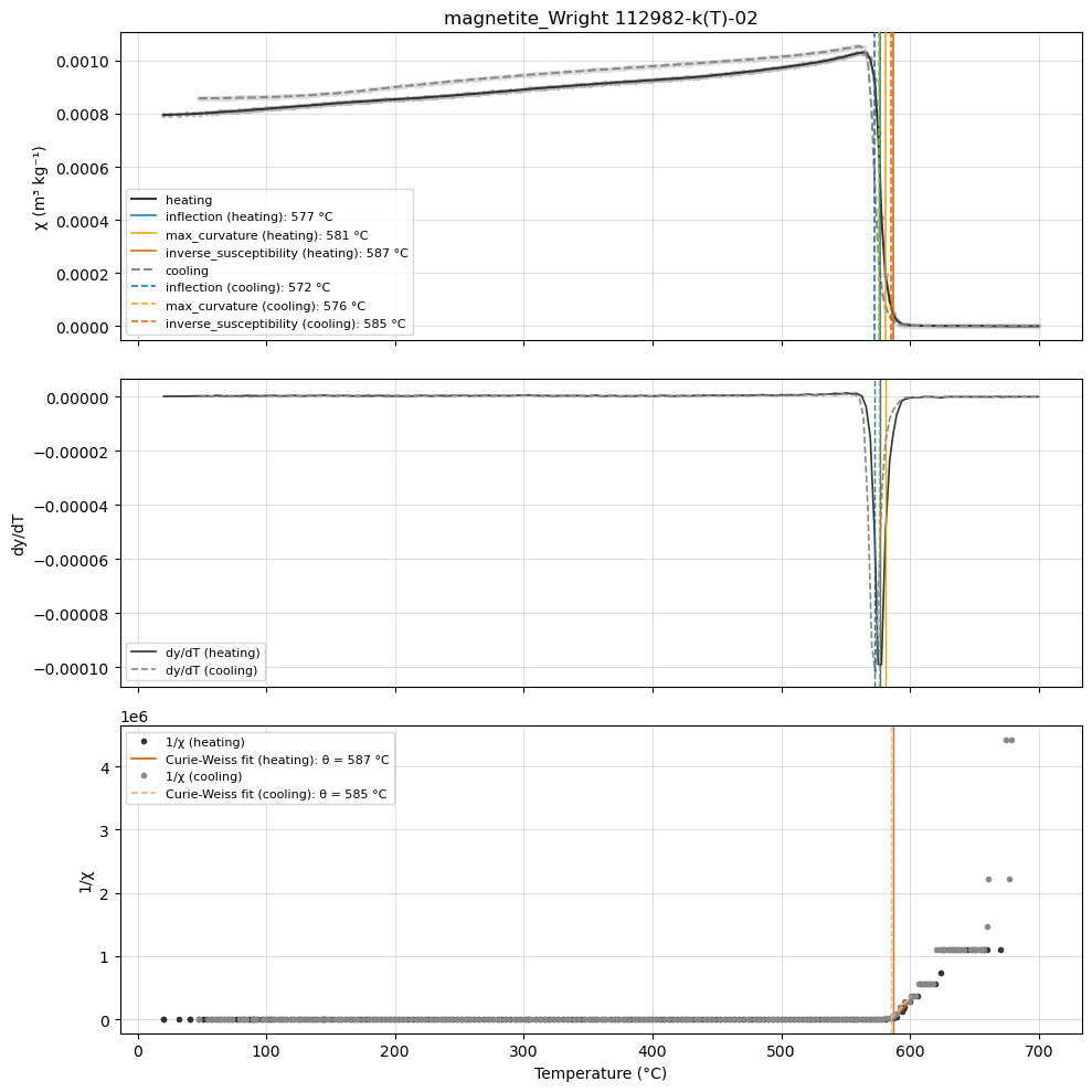
The full measured range puts the transition in context, but the estimates themselves span only a few tens of degrees. Passing xlim zooms all panels in on the transition (they share the temperature axis), and each panel’s y axis autoscales to the data within the window — note how the 1/ panel below resolves the Curie-Weiss fit that is compressed against zero in the full-range view above. Pass ylim to set the main panel’s y limits explicitly. The main-panel legend sits at the lower left by default, where thermomagnetic curves rarely reach; if it collides with data on a particular curve, move it with legend_loc (any matplotlib legend location string).
rmag.plot_curie_estimates(
    selected_experiment,
    smooth_window=10,
    method_kwargs={'inverse_susceptibility': {'fit_range': (586, 604)}},
    figsize=(10, 10),
    xlim=(540, 620),
);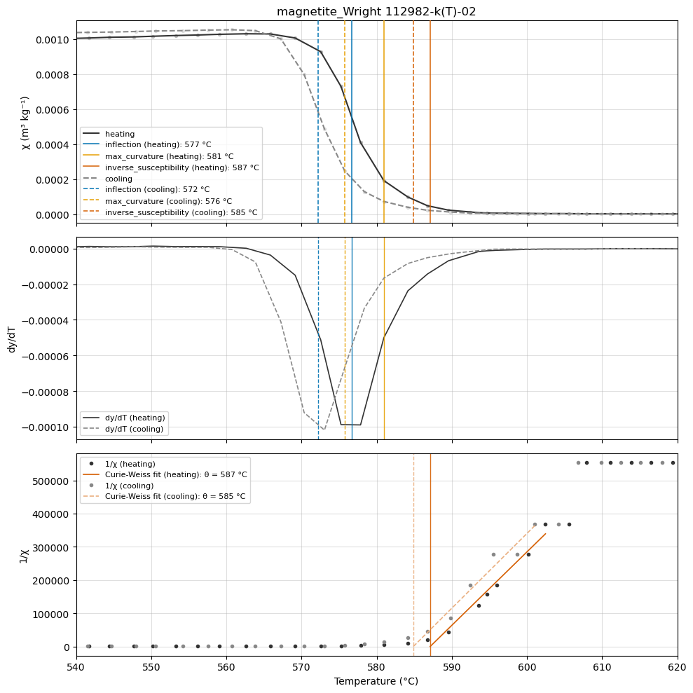
The heating-branch inflection (~577 °C) and maximum-curvature (~581 °C) estimates bracket the accepted magnetite Curie temperature of 580 °C. The steep, step-like decrease of (T) at the transition in a (near-)multidomain magnetite is dominated by the loss of the self-demagnetization-limited susceptibility plateau, and for such curves the derivative-based estimates on the descending step are close to T (Fabian et al., 2013). The Curie-Weiss fit over the resolved 585–606 °C interval yields 587 ± 1 °C, consistent with the requirement T and with exceeding T by several degrees for a ferrimagnet. The cooling-branch estimates differ from the heating branch by a few degrees; larger heating-cooling differences (irreversibility) signal alteration of the magnetic mineralogy during heating, in which case the cooling branch reflects the altered assemblage, not the original one.
The two-tangent construction on (T): shown only to be discouraged
Requesting two_tangent on susceptibility data attaches the caveat to the output. On this curve the two-tangent intersection lands close to the derivative estimates because the transition is sharp, but on curves with a pronounced Hopkinson peak or a rounded transition it can overestimate T considerably (Petrovský and Kapička, 2006) — and there is no physical justification for it on low-field susceptibility even when it happens to agree.
two_tangent_chi = rmag.curie_temperature_estimates(
    selected_experiment, methods=('two_tangent',), smooth_window=10)
two_tangent_chi[['branch', 'method', 'curie_temp', 'notes']]Interactive Curie-Weiss fitting
The draggable fit tool below helps identify the temperature interval over which 1/ is linear (i.e., where the signal is fully paramagnetic): drag the two endpoints and the extrapolated updates live. This tool is for exploration; for reported values, feed the interval identified here to curie_inverse_susceptibility (or the method_kwargs of curie_temperature_estimates) so the fit is reproducible.
rmag.curie_inverse_susceptibility_interactive(
    selected_experiment,
    smooth_window=10,
    initial_fit_range=(585, 606),
)A Curie transition inside the MPMS window: titanomagnetite TM78
For titanomagnetite compositions with x 0.75, the Curie temperature falls below room temperature, and the entire transition is captured by low-temperature MPMS susceptibility measurements. The TM78 sample from the Rock Magnetic Bestiary shows the susceptibility rising through a Hopkinson-like peak and collapsing near 265 K. The same estimator functions apply — only the temperature range differs.
Note remove_holder=False here: the default holder correction subtracts the per-branch minimum, which assumes the signal decays to a background level at the highest temperatures. For this specimen the branch minimum is the still-substantial paramagnetic susceptibility above the transition, not a holder background, so subtracting it would distort the curve.
tm78_experiment = measurements[(measurements['experiment'] ==
                                'IRM-OldBlue-LP-X:LP-X-T:LP-X-F:LP-X-H-9764')].reset_index(drop=True)
# use the 1 Hz in-phase susceptibility
tm78_1hz = tm78_experiment[np.isclose(tm78_experiment['meas_freq'].astype(float), 1.0)].reset_index(drop=True)

tm78_estimates = rmag.curie_temperature_estimates(
    tm78_1hz, temp_unit='K', methods=('inflection', 'max_curvature'), remove_holder=False)
tm78_estimates[['branch', 'method', 'curie_temp', 'temp_unit']]rmag.plot_curie_estimates(tm78_1hz, temp_unit='K', methods=('inflection', 'max_curvature'),
remove_holder=False, figsize=(10, 7));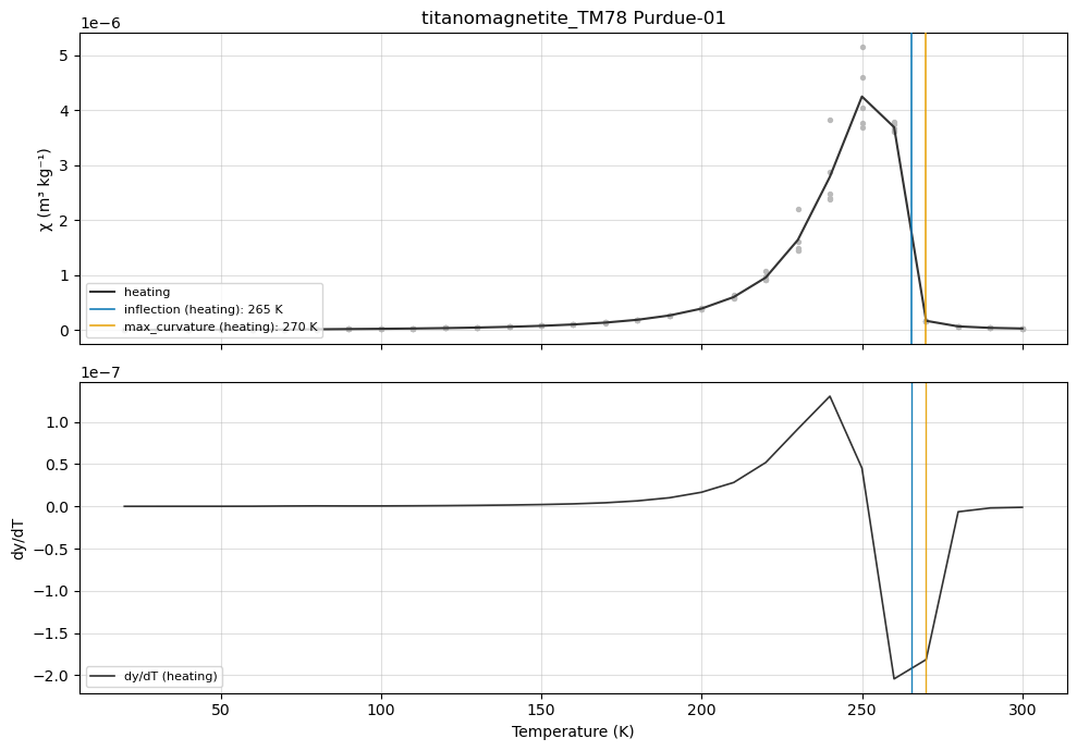
Part 3: Archiving the estimate in a MagIC specimens table
The MagIC data model stores critical temperatures in the specimens table: critical_temp (in kelvin) with critical_temp_type from the controlled vocabulary (here 'Curie'). rmag.add_curie_estimates_to_specimens_table writes the chosen estimate and records the estimation method, branch, and uncertainty in the description column, so that the processing choice is archived with the result.
Rows are matched on the specimens table’s experiments column, which in this contribution abbreviates the experiment name to 'IRM-KappaF-3410' (the measurements table uses the longer 'IRM-KappaF-LP-X-T-3410'), so we pass the name as it appears in the specimens table. If no experiment name matches, the function falls back to matching the specimen name and warns.
This contribution already archives a critical temperature for this specimen (849.70 K from a d/dT minimum on heating): our heating-branch inflection estimate of 849.82 K (576.7 °C) reproduces it to within ~0.1 K, a satisfying independent check before overwriting the row.
specimens = contribution.tables['specimens'].df.reset_index(drop=True)

rmag.add_curie_estimates_to_specimens_table(
    specimens,
    experiment_name='IRM-KappaF-3410',
    estimates=curie_estimates,
    method='inflection',
    branch='heating',
)
specimens[specimens['specimen'] == 'magnetite_Wright 112982-k(T)-02'][
['specimen', 'experiments', 'critical_temp', 'critical_temp_type', 'description']]Summary
Curie temperature estimates are method-dependent; report the method (and any smoothing/fitting windows) with the value.
For in-field M(T) curves: the inflection point is the physically grounded estimate; maximum-curvature and two-tangent values run systematically high; the Landau fit adds a formal uncertainty; for runs that end below T, the M extrapolation of Moskowitz (1981) is available, with reliability decaying as the gap to T grows.
For (T) curves: derivative-based estimates on the descending step and the inverse-susceptibility (Curie-Weiss) extrapolation are appropriate; the two-tangent construction is not; and from 1/ is an upper bound on T.
Comparing estimates across methods (and between heating and cooling branches) is itself diagnostic — of T distributions, alteration, and data quality.
References
Ade-Hall, J., Wilson, R., and Smith, P. (1965), The petrology, Curie points and natural magnetizations of basic lavas, Geophysical Journal International, 9, 323-336.
Fabian, K., Shcherbakov, V. P., and McEnroe, S. A. (2013), Measuring the Curie temperature, Geochemistry, Geophysics, Geosystems, 14, 947-961, Fabian et al. (2013).
Grommé, C. S., Wright, T. L., and Peck, D. L. (1969), Magnetic properties and oxidation of iron-titanium oxide minerals in Alae and Makaopuhi lava lakes, Hawaii, Journal of Geophysical Research, 74, 5277-5294, Grommé et al. (1969).
Lattard, D., Engelmann, R., Kontny, A., and Sauerzapf, U. (2006), Curie temperatures of synthetic titanomagnetites in the Fe-Ti-O system: Effects of composition, crystal chemistry, and thermomagnetic methods, Journal of Geophysical Research, 111, B12S28, Lattard et al. (2006).
Moskowitz, B. M. (1981), Methods for estimating Curie temperatures of titanomaghemites from experimental Js-T data, Earth and Planetary Science Letters, 53, 84-88, Moskowitz (1981).
Petrovský, E., and Kapička, A. (2006), On determination of the Curie point from thermomagnetic curves, Journal of Geophysical Research, 111, B12S27, Petrovský & Kapička (2006).
- Lattard, D., Engelmann, R., Kontny, A., & Sauerzapf, U. (2006). Curie temperatures of synthetic titanomagnetites in the Fe-Ti-O system: Effects of composition, crystal chemistry, and thermomagnetic methods. Journal of Geophysical Research: Solid Earth, 111, B12S28. 10.1029/2006JB004591
- Fabian, K., Shcherbakov, V. P., & McEnroe, S. A. (2013). Measuring the Curie temperature. Geochemistry, Geophysics, Geosystems, 14(4), 947–961. 10.1029/2012GC004440
- Grommé, C. S., Wright, T. L., & Peck, D. L. (1969). Magnetic properties and oxidation of iron-titanium oxide minerals in Alae and Makaopuhi Lava Lakes, Hawaii. Journal of Geophysical Research, 74(22), 5277–5294. 10.1029/JB074i022p05277
- Petrovský, E., & Kapička, A. (2006). On determination of the Curie point from thermomagnetic curves. Journal of Geophysical Research: Solid Earth, 111, B12S27. 10.1029/2006JB004507
- Moskowitz, B. M. (1981). Methods for estimating Curie temperatures of titanomaghemites from experimental Js-T data. Earth and Planetary Science Letters, 53(1), 84–88. 10.1016/0012-821X(81)90028-5