FORC data analysis - RockmagPy Documentation

First-order reversal curve (FORC) diagrams map the joint distribution of switching fields and interaction fields within an assemblage of magnetic particles, providing insight into domain state and magnetostatic interactions and resolving components that bulk hysteresis parameters average together (Roberts et al., 2000; Roberts et al., 2014).

A FORC is a partial hysteresis curve within the interior of the major loop. The specimen is saturated, the field is lowered along the descending branch to a reversal field H_a, and the magnetization is then measured at increasing applied fields H_b as the field returns to saturation (Figure 1a). Repeating this for successively lower reversal fields fills the loop with many curves (Figure 1b) that together define a magnetization surface M(H_a, H_b) on the half-plane H_b ≥ H_a (Figure 1c). The FORC distribution is the mixed second derivative of that surface (Figure 1d).

What a FORC measurement is and how the distribution follows from it, shown with the Baraboo hematite vein material example distributed with RockmagPy (measured by Maxwell Brown at the IRM). Moments are in absolute units throughout: this specimen does not reach saturation within the measured field range, so there is no meaningful Ms to normalize by. (a) One reversal curve (blue) within the major hysteresis loop (grey). The curve departs the descending branch at the reversal field Ha (open circle) and is measured with increasing applied field Hb; each measurement is one value M(Ha, Hb) of the surface (red), where Ha identifies the curve as a whole and Hb the position along it. (b) All of the first-order reversal curves in this dataset. (c) The individual measurements plotted at their own (Hb, Ha) and colored by moment. Each reversal curve is one horizontal row of points, and data exist only where Hb ≥ Ha, so they fill a half-plane bounded by the diagonal. The rows stop at Ha = +95 mT, the highest reversal field used, because reversing from a field above the switching range simply retraces the descending branch and contributes nothing to ρ. The sloping edge on the right is a line of constant Bu = 100 mT: this acquisition set a bias-field window, recorded in the file header as Hb2 = +0.1 T, and every curve terminates there. The left-to-right gradient is the high-field slope, which carries no information about ρ. (d) The FORC distribution ρ = −½ ∂²M/∂Ha∂Hb on those same axes, estimated by local quadratic regression. The rotated coordinates in which FORC diagrams are conventionally drawn are overlaid as arrows. Bu runs parallel to the diagonal and Bc at right angles to it, so the diagonal Hb = Ha is simultaneously the edge of the measured region and the Bc = 0 axis. 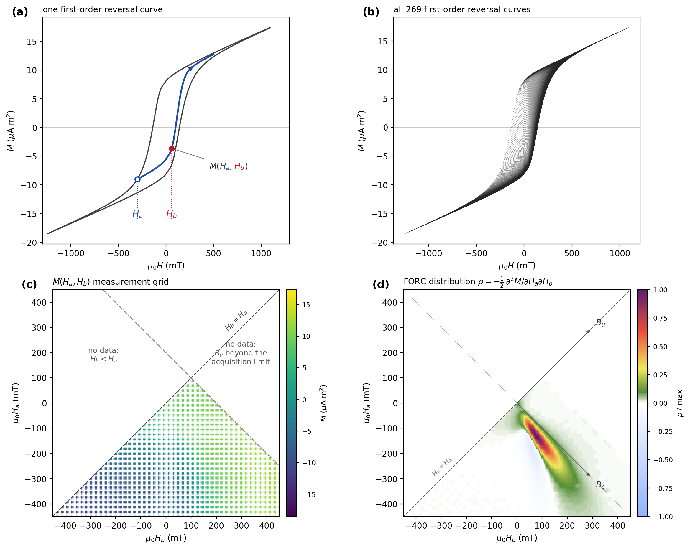— Figure 1:What a FORC measurement is and how the distribution follows from it, shown with the Baraboo hematite vein material example distributed with RockmagPy (measured by Maxwell Brown at the IRM). Moments are in absolute units throughout: this specimen does not reach saturation within the measured field range, so there is no meaningful M_s to normalize by. (a) One reversal curve (blue) within the major hysteresis loop (grey). The curve departs the descending branch at the reversal field H_a (open circle) and is measured with increasing applied field H_b; each measurement is one value M(H_a, H_b) of the surface (red), where H_a identifies the curve as a whole and H_b the position along it. (b) All of the first-order reversal curves in this dataset. (c) The individual measurements plotted at their own (H_b, H_a) and colored by moment. Each reversal curve is one horizontal row of points, and data exist only where H_b ≥ H_a, so they fill a half-plane bounded by the diagonal. The rows stop at H_a = +95 mT, the highest reversal field used, because reversing from a field above the switching range simply retraces the descending branch and contributes nothing to ρ. The sloping edge on the right is a line of constant B_u = 100 mT: this acquisition set a bias-field window, recorded in the file header as `Hb2` = +0.1 T, and every curve terminates there. The left-to-right gradient is the high-field slope, which carries no information about ρ. (d) The FORC distribution ρ = −½ ∂²M/∂H_a∂H_b on those same axes, estimated by local quadratic regression. The rotated coordinates in which FORC diagrams are conventionally drawn are overlaid as arrows. B_u runs parallel to the diagonal and B_c at right angles to it, so the diagonal H_b = H_a is simultaneously the edge of the measured region and the B_c = 0 axis.

FORC Processing This notebook shows the standard RockmagPy FORC workflow showing: a diagram, profiles, and a ridge-following profile. It works through what the processing does: reading raw Lake Shore (Princeton MicroMag) VSM files, drift correction, archiving to the MagIC data model, and calculation of the FORC distribution. It also covers the marginal coercivity distribution — the FORC distribution collapsed along the bias axis, which can be compared with backfield-derived coercivity spectra. We also describe how the implementation compares to other available tools including: FORCinel, VARIFORC and FORCsensei.
FORC Smoothing Smoothing is a quite consequential analytical choice in FORC processing. This notebook gives a practical recipe for choosing a level, then illustrates what the local-regression neighborhood is, how much of it is usable near the B_c = 0 axis, what over- and under-smoothing do to a feature of known width, a residual-based selection criterion of the kind FORCinel uses, and why a single smoothing window cannot serve a narrow ridge and a broad background at once. We also show comparisons for the same data on different color scales that influence.
VARIFORC variable smoothing A single smoothing window cannot resolve a narrow ridge and suppress a broad background at the same time. This notebook applies the variable-smoothing protocol of Egli (2013) as implemented in RockmagPy to a magnetofossil-bearing carbonate carrying a central ridge, shows how the regression window varies across the diagram, uses the per-cell uncertainty of Heslop and Roberts (2012) to identify which parts of a diagram the data support, and checks the implementation against Egli’s published resolution law and against the independent FORCsensei implementation of VARIFORC.

Field conventions¶

The notebooks and pmagpy.forc follow the conventions of Pike et al. (1999) and the subsequent FORC literature:

H_a is the reversal field at which a curve begins (the open circle in Figure 1a).
H_b is the applied field along that curve, with H_b ≥ H_a — the constraint that confines the data to the half-plane above the diagonal in Figure 1c.
The FORC distribution is ρ(H_a, H_b) = −½ ∂²M/∂H_a∂H_b (Figure 1d).
Diagrams are drawn in the rotated coordinates B_c = (H_b − H_a)/2 (coercivity) and B_u = (H_b + H_a)/2 (interaction/bias field), overlaid as arrows in Figure 1d.

Fields are handled in tesla and moments in Am² throughout. Files recorded in cgs (Oe, emu) are converted when they are imported.

Be aware that MicroMag file headers use Hb1/Hb2 and Hc1/Hc2 for something else entirely — the display bounds of the diagram, not reversal and applied fields. The sloping right-hand edge in Figure 1c is the imprint of one such bound (Hb2) on the measured data. FORC_processing.ipynb covers how these are read.

A note on smoothing¶

Because ρ is obtained by twice differentiating measured magnetization data, smoothing is an important part of the calculation and the smoothing chosen is a consequential analytical choice in FORC processing. pmagpy.forc sets an initial level automatically from the geometry of the measurement and records it, with every other processing decision, in the output. The choices made for smoothing need to be documented and presented for any presented FORC diagram.

FORC_smoothing.ipynb works through the importance of smoothing and illustrates the effect of different smoothing choices; FORC_variforc.ipynb covers the case where the data would be better treated by variable smoothing instead of a single level.

Archiving FORC measurements¶

pmagpy.forc enables the export of raw instrument files to a MagIC measurements table under the LP-FORC method code. Archiving the reversal curves themselves keeps the full processing chain including drift correction, smoothing choices, and the resulting distribution to be reproduced and revisited with different processing approaches.

References¶

Roberts, A. P., Pike, C. R., & Verosub, K. L. (2000). First‐order reversal curve diagrams: A new tool for characterizing the magnetic properties of natural samples. Journal of Geophysical Research: Solid Earth, 105(B12), 28461–28475. 10.1029/2000jb900326
Roberts, A. P., Heslop, D., Zhao, X., & Pike, C. R. (2014). Understanding fine magnetic particle systems through use of first-order reversal curve diagrams: FORC diagrams. Reviews of Geophysics, 52(4), 557–602. 10.1002/2014rg000462
Harrison, R. J., & Feinberg, J. M. (2008). FORCinel: An improved algorithm for calculating first‐order reversal curve distributions using locally weighted regression smoothing. Geochemistry, Geophysics, Geosystems, 9(5). 10.1029/2008gc001987
Egli, R. (2013). VARIFORC: An optimized protocol for calculating non-regular first-order reversal curve (FORC) diagrams. Global and Planetary Change, 110, 302–320. 10.1016/j.gloplacha.2013.08.003
Heslop, D., Roberts, A. P., Oda, H., Zhao, X., Harrison, R. J., Muxworthy, A. R., Hu, P. ‐X., & Sato, T. (2020). An Automatic Model Selection‐Based Machine Learning Framework to Estimate FORC Distributions. Journal of Geophysical Research: Solid Earth, 125(10). 10.1029/2020jb020418
Heslop, D., & Roberts, A. P. (2012). Estimation of significance levels and confidence intervals for first‐order reversal curve distributions. Geochemistry, Geophysics, Geosystems, 13(5). 10.1029/2012gc004115
Pike, C. R., Roberts, A. P., & Verosub, K. L. (1999). Characterizing interactions in fine magnetic particle systems using first order reversal curves. Journal of Applied Physics, 85(9), 6660–6667. 10.1063/1.370176