A single smoothing window is a compromise whenever a FORC diagram carries features on different scales at once, which is the normal case: a narrow ridge sitting on a broad, low-amplitude background. Resolve the ridge and the background is noise; clean the background and the ridge is smeared.
The variable-smoothing protocol of
Egli (2013) removes the compromise. It
lets the regression window grow with distance from the origin of the diagram, where
Preisach-type FORC functions genuinely are smoother, while holding it narrow across the
features that need resolving. pmagpy.forc implements it, together with the per-cell
error analysis of Heslop and Roberts (2012).
This notebook leads with the workflow and then works through it:
The workflow: variable smoothing on a magnetofossil sample in one call.
What changes and why: conventional versus variable smoothing side by side.
How the window varies across the diagram.
Significance: which parts of a diagram the data actually support.
Choosing parameters for your own sample.
Diagonal artefacts and how they are suppressed.
Fidelity: how the implementation is checked against the published algorithm.
It builds on FORC
Example data. The measurements used here are redistributed from the example datasets that accompany the VARIFORC package, with thanks to Ramon Egli. See
SOURCE.mdfor provenance and licensing. The implementation inpmagpy.forcis independent, written from the published equations rather than from the VARIFORC source.
Install and import packages
import numpy as np
import matplotlib.pyplot as plt

import pmagpy.forc as forc

%matplotlib inline
%config InlineBackend.figure_format = 'retina'

print(f"compiled fast path available: {forc.numba_available()}")
compiled fast path available: True
1. The workflow
The sample is a magnetofossil-bearing pelagic carbonate from the Eastern Equatorial Pacific: 450 reversal curves at 0.5 mT on an alternating gradient magnetometer. Its diagnostic feature is a central ridge — a horizontal ridge along Bu = 0 that is the signature of non-interacting single-domain particles (Egli et al., 2010). A central ridge is intrinsically narrow in Bu, so it is exactly the feature that oversmoothing destroys.
variforc_settings describes the sample by what its diagram shows rather than by
smoothing factors. Here: a central ridge, sitting a few tenths of a millitesla above the
axis, on a background that can take a much larger window.
data = '../example_data/FORC/variforc_examples/magnetofossil_S0_a.txt'

settings = forc.variforc_settings(
    'central_ridge',              # what the diagram shows
    smoothing_factor=9,           # baseline window away from the ridge
    growth_rate=0.1,              # how fast it grows with distance
    central_ridge=4,              # window held this narrow across the ridge
    central_ridge_position=0.0004,  # the ridge sits 0.4 mT above Bu = 0
)

out = forc.process_forc(
    mode='i', path=data,
    do_regrid=True, B_step=0.0005,
    smoothing='variforc', variforc=settings,
    Bu_min=-0.10, Bu_max=0.06, Bc_max=0.12,
    color_scale_version=2, plot_hyst=False, verbose=False,
)
OMP: Info #276: omp_set_nested routine deprecated, please use omp_set_max_active_levels instead.
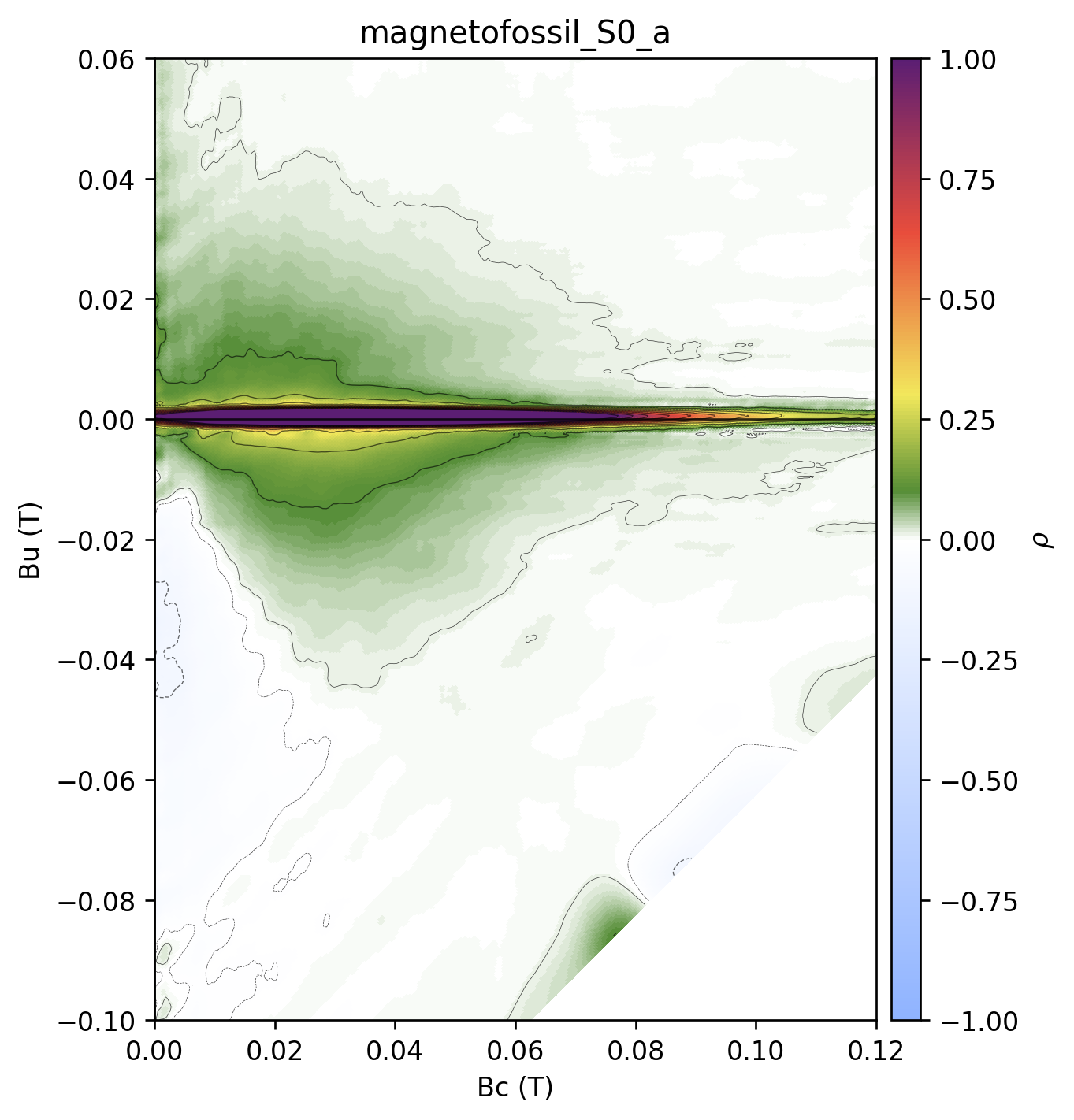
The central ridge is resolved sharply while the background is smooth enough to contour. Everything used is recorded with the result.
params = out['smoothing_params']
print(f"method            : {params['method']} (preset {params['preset']!r})")
print(f"baseline factor   : s1 = {params['sc1']:g}, growth rate lambda = "
      f"{params['lambda_c']:g}")
print(f"ridge floor       : s_b0 = {params['sb0']:g}")
print(f"calibration points: {out['n_calibration_points']}, "
      f"drift corrected: {out['drift_corrected']}")
method : variforc (preset 'central_ridge')
baseline factor : s1 = 9, growth rate lambda = 0.1
ridge floor : s_b0 = 4
calibration points: 450, drift corrected: True
2. What changes, and why
The clearest way to see what variable smoothing buys is to put it beside conventional processing at two fixed smoothing factors: one small enough to resolve the ridge, and one large enough to clean the background.
Ha, Hb = out['Ha_vals_used'], out['Hb_vals_used']
M = out['M_grid_used']
Bu, Bc = forc.bu_bc_from_ha_hb(Ha, Hb)
Ha_e, Hb_e = np.meshgrid(forc.centers_to_edges(Ha),
                         forc.centers_to_edges(Hb), indexing='ij')
Bc_e, Bu_e = 0.5 * (Hb_e - Ha_e), 0.5 * (Hb_e + Ha_e)
window = (Bc >= 0) & (Bc <= 0.12) & (Bu >= -0.10) & (Bu <= 0.06)

variants = [
    ('conventional SF = 4\n(resolves the ridge)',
     dict(sc0=5, sc1=5, sb0=5, sb1=5, lambda_c=0.0, lambda_b=0.0)),
    ('conventional SF = 10\n(cleans the background)',
     dict(sc0=11, sc1=11, sb0=11, sb1=11, lambda_c=0.0, lambda_b=0.0)),
    ('variable smoothing\n(does both)', settings),
]

fig, axes = plt.subplots(2, 3, figsize=(13, 6.6), constrained_layout=True,
                         height_ratios=[2, 1])
for k, (title, kw) in enumerate(variants):
    rho = forc.variforc_rho_from_grid(Ha, Hb, M, min_pts=8, **kw)
    vmax = np.nanpercentile(np.abs(rho[window & np.isfinite(rho)]), 99.0)

    ax = axes[0, k]
    ax.pcolormesh(1e3 * Bc_e, 1e3 * Bu_e, rho / vmax, cmap=forc.get_forc_cmap(2),
                  vmin=-1, vmax=1, shading='auto', rasterized=True)
    ax.set_xlim(0, 120); ax.set_ylim(-100, 60)
    ax.axhline(0, color='k', lw=0.4, alpha=0.5)
    ax.set_title(title, fontsize=9, loc='left')
    ax.set_xlabel(r'$B_c$ (mT)')
    if k == 0:
        ax.set_ylabel(r'$B_u$ (mT)')

    # vertical profile across the ridge
    band = (Bc > 0.02) & (Bc < 0.05) & (np.abs(Bu) < 0.015) & np.isfinite(rho)
    centres, profile = forc.bin_profile(Bu[band], rho[band], -0.015, 0.015,
                                        n_bins=120)
    peak = forc.profile_peak_and_fwhm(centres, profile, use_abs=False)
    background = (np.abs(Bu) > 0.03) & (Bc > 0.05) & (Bc < 0.10) & np.isfinite(rho)

    ax = axes[1, k]
    ax.plot(1e3 * centres, profile / np.nanmax(profile), 'k-', lw=1.2)
    ax.axvline(0, color='0.8', lw=0.6)
    ax.set_xlim(-15, 15); ax.set_ylim(-0.25, 1.1)
    ax.set_xlabel(r'$B_u$ (mT)')
    if k == 0:
        ax.set_ylabel(r'$\rho$ / max')
    ax.set_title(f"ridge FWHM {1e3 * peak['fwhm']:.2f} mT, "
                 f"background {np.nanstd(rho[background]) / np.nanmax(rho[window & np.isfinite(rho)]):.2%}",
                 fontsize=8.5, loc='left')
plt.show()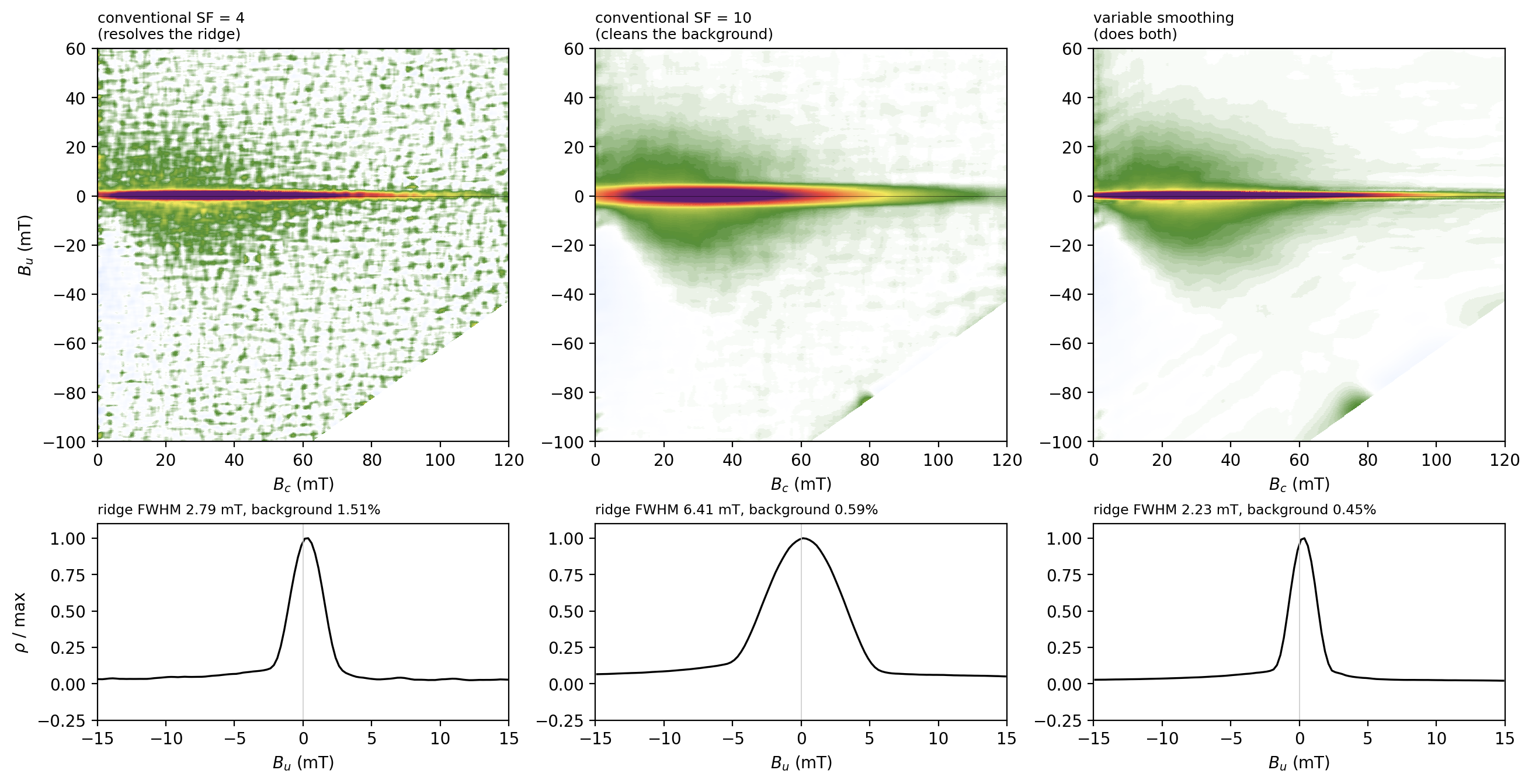
The two conventional panels show the trade-off directly: the small window keeps the ridge narrow but leaves a speckled background, while the large window cleans the background and roughly doubles the apparent ridge width. Variable smoothing gives the narrowest ridge of the three and the quietest background, because it uses a different window in each place.
That the ridge should be this narrow is the scientific point. Its width in Bu is what distinguishes non-interacting single-domain particles from a weakly interacting assemblage, so a processing choice that broadens it changes the interpretation.
3. How the window varies
The smoothing factors are not free parameters chosen per cell; they follow Egli’s rule,
The first term grows the window linearly away from the origin. The second holds it at a floor across a ridge, then relaxes just fast enough that a window centred near the ridge never reaches across it.
result = forc.variforc_rho_from_grid(Ha, Hb, M, min_pts=8,
                                     return_factors=True, **settings)

fig, axes = plt.subplots(1, 2, figsize=(11, 3.6), constrained_layout=True)
for ax, key, label in ((axes[0], 's_c', r'horizontal factor $s_c$'),
                       (axes[1], 's_b', r'vertical factor $s_b$')):
    mesh = ax.pcolormesh(1e3 * Bc_e, 1e3 * Bu_e, result[key], cmap='viridis',
                         shading='auto', rasterized=True)
    ax.set_xlim(0, 120); ax.set_ylim(-100, 60)
    ax.set_xlabel(r'$B_c$ (mT)')
    ax.set_ylabel(r'$B_u$ (mT)')
    ax.set_title(label, fontsize=9, loc='left')
    fig.colorbar(mesh, ax=ax, label='window half-width (field steps)')
plt.show()

print(f"s_c ranges {result['s_c'].min():.1f} to {result['s_c'].max():.1f} field steps")
print(f"s_b ranges {result['s_b'].min():.1f} to {result['s_b'].max():.1f} field steps")
print(f"the narrow horizontal band in s_b is the central ridge, held at "
      f"{settings['sb0']:g}")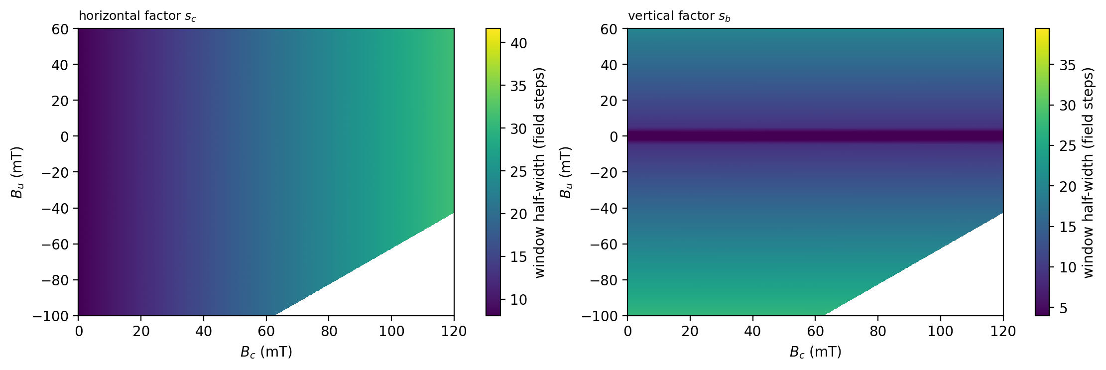
s_c ranges 8.1 to 41.6 field steps
s_b ranges 4.0 to 39.4 field steps
the narrow horizontal band in s_b is the central ridge, held at 4
The vertical factor is pinned to its floor in a narrow band along the ridge and grows away from it; the horizontal factor grows steadily with coercivity. Away from the ridge the window reaches several tens of field steps, which is why the background is so much quieter than conventional processing at any factor small enough to keep the ridge sharp.
4. Which parts of the diagram the data support
Growing the window widens the region that is statistically significant, which is the other
half of Egli’s argument. With estimate_uncertainty=True the measurement noise is
propagated through each local fit to a standard error on ρ, following Heslop and Roberts
(2012). The signal-to-noise ratio then says which features are real.
significance = {}
for label, s in (('conventional SF = 4',
                  dict(sc0=5, sc1=5, sb0=5, sb1=5, lambda_c=0.0, lambda_b=0.0)),
                 ('variable smoothing', settings)):
    res = forc.variforc_rho_from_grid(Ha, Hb, M, min_pts=8,
                                      estimate_uncertainty=True, **s)
    significance[label] = res

fig, axes = plt.subplots(1, 2, figsize=(11, 3.6), constrained_layout=True)
for ax, (label, res) in zip(axes, significance.items()):
    snr = res['snr']
    mesh = ax.pcolormesh(1e3 * Bc_e, 1e3 * Bu_e, snr, cmap='magma',
                         vmin=0, vmax=30, shading='auto', rasterized=True)
    ax.contour(1e3 * Bc, 1e3 * Bu, snr, levels=[3.0], colors='c', linewidths=0.8)
    ax.set_xlim(0, 120); ax.set_ylim(-100, 60)
    ax.set_xlabel(r'$B_c$ (mT)')
    ax.set_title(label, fontsize=9, loc='left')
    fig.colorbar(mesh, ax=ax, label='signal-to-noise ratio')
    inside = window & np.isfinite(snr)
    print(f"{label:22s} noise {res['noise']:.2e} A m$^2$, "
          f"{np.mean(snr[inside] > 3):.0%} of the plotted window has SNR > 3")
axes[0].set_ylabel(r'$B_u$ (mT)')
plt.show()
conventional SF = 4 noise 5.40e-11 A m$^2$, 50% of the plotted window has SNR > 3
variable smoothing noise 5.40e-11 A m$^2$, 91% of the plotted window has SNR > 3
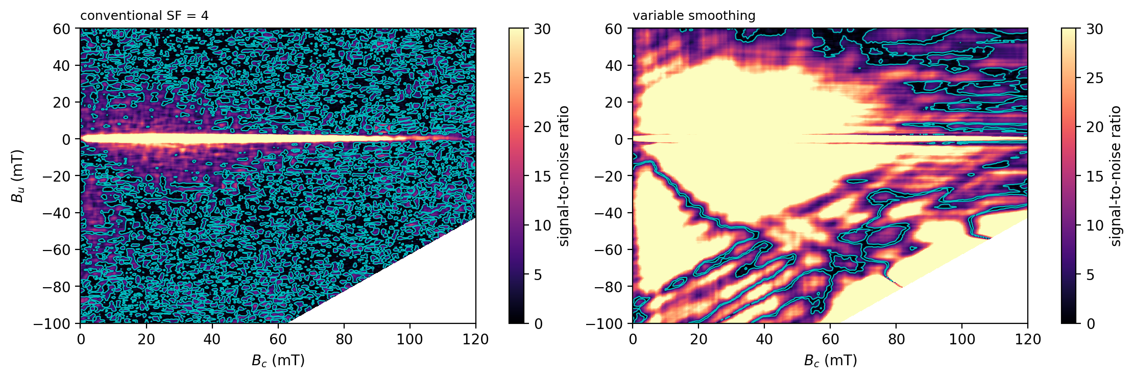
The cyan contour is the SNR = 3 significance threshold. Variable smoothing extends the significant region over a much larger part of the diagram, so features in the background can be interpreted rather than dismissed as noise. Egli treats SNR > 3 as the threshold for a contribution being distinguishable from zero, and suggests contours are only worth drawing where the SNR is comfortably above it.
5. Choosing parameters for your own sample
Four presets cover the cases Egli distinguishes, keyed to what a conventionally processed diagram shows.
for name, meta in forc.VARIFORC_PRESETS.items():
    print(f"{name:16s} {meta['description']}")
regular No sharp ridges: a smooth Preisach-type distribution.
central_ridge A horizontal ridge along Bu = 0, the signature of non-interacting single-domain particles such as magnetofossils.
vertical_ridge A vertical ridge along Bc = 0, produced by thermal relaxation in superparamagnetic assemblages.
both_ridges Both a central and a vertical ridge over a continuous background, as in many volcanic ash and pseudo-single-domain samples.
Two numbers then matter:
smoothing_factorsets the baseline window away from any ridge. Egli’s published analyses use 7 to 11. Larger suppresses more noise.growth_ratesets how fast the window grows with distance from the origin. Between about 0.06 and 0.12 is sensible; 0 reproduces conventional processing. Above roughly 0.2 the windows become large enough to create their own artefacts, which is what the diagonal limits in section 6 exist to control.
The practical recipe is unchanged from conventional processing: compute at several settings, keep the features that persist, and report what you used.
fig, axes = plt.subplots(1, 4, figsize=(14, 3.2), constrained_layout=True, sharey=True)
for ax, growth in zip(axes, (0.0, 0.05, 0.10, 0.15)):
    trial = forc.variforc_settings('central_ridge', smoothing_factor=9,
                                   growth_rate=growth, central_ridge=4,
                                   central_ridge_position=0.0004)
    rho = forc.variforc_rho_from_grid(Ha, Hb, M, min_pts=8, **trial)
    vmax = np.nanpercentile(np.abs(rho[window & np.isfinite(rho)]), 99.0)
    ax.pcolormesh(1e3 * Bc_e, 1e3 * Bu_e, rho / vmax, cmap=forc.get_forc_cmap(2),
                  vmin=-1, vmax=1, shading='auto', rasterized=True)
    ax.set_xlim(0, 120); ax.set_ylim(-100, 60)
    ax.set_xlabel(r'$B_c$ (mT)')
    ax.set_title(f'growth rate = {growth}', fontsize=9, loc='left')
axes[0].set_ylabel(r'$B_u$ (mT)')
plt.show()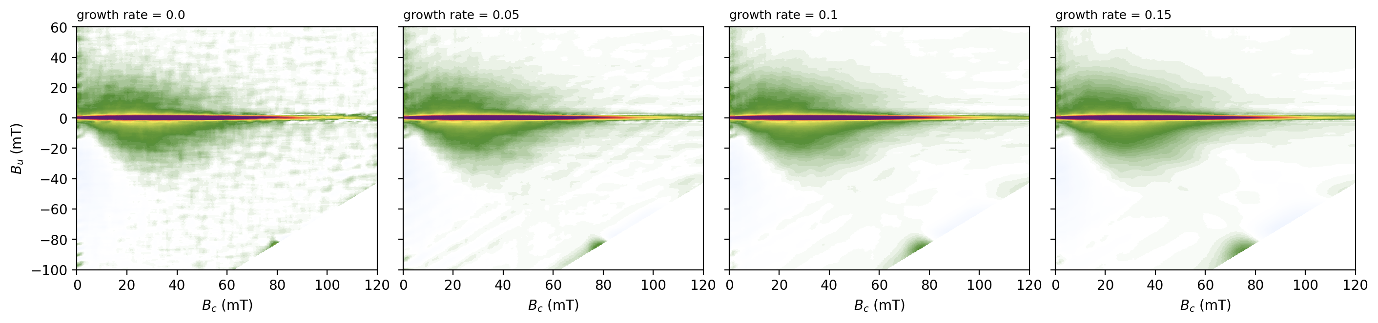
6. Diagonal artefacts
Large regression windows misfit where the measured curves change most sharply: where the curves are steepest, and where consecutive curves differ most. In FORC coordinates those conditions fall along the two diagonals through the coercive field, and a window spanning them produces ridge-like artefacts that are not features of the sample.
Egli’s remedy is not to shrink the window, which would trade one artefact for another, but to truncate its corners along 45° lines so that the rectangle becomes an octagon narrow enough in the diagonal direction while keeping its resolution along Bc and Bu.
Cultured magnetotactic bacteria have a near-rectangular hysteresis loop and show the problem clearly.
bacteria = '../example_data/FORC/variforc_examples/magnetotactic_MV1.txt'
segs, _ = forc.phase1_prepare_segments_dual(bacteria, export_magic=False, verbose=False)
curves = [s for s in segs if s.kind == 'forc']
step = forc.infer_B_step_from_forcs(curves)
curves = forc.regrid_forcs_in_hysteresis_space(curves, B_step=step, verbose=False)
Ha2, Hb2, M2, _, _ = forc.build_forc_grid(curves, verbose=False)
Bu2, Bc2 = forc.bu_bc_from_ha_hb(Ha2, Hb2)
Ha2_e, Hb2_e = np.meshgrid(forc.centers_to_edges(Ha2),
                           forc.centers_to_edges(Hb2), indexing='ij')
Bc2_e, Bu2_e = 0.5 * (Hb2_e - Ha2_e), 0.5 * (Hb2_e + Ha2_e)
win2 = (Bc2 >= 0) & (Bc2 <= 0.10) & (Bu2 >= -0.08) & (Bu2 <= 0.05)

print(f"estimated coercive field: {1e3 * forc.find_coercive_field(Ha2, Hb2, M2):.1f} mT")

base = dict(sc0=9, sc1=9, sb0=3, sb1=9, lambda_c=0.1, lambda_b=0.1,
            ridge_limits=[('Bu', 0.0003, 3, 0.0004)])
fig, axes = plt.subplots(1, 2, figsize=(10, 3.8), constrained_layout=True)
for ax, (title, extra) in zip(axes, [
        ('no diagonal limit', {}),
        ('corners truncated (Egli INPUT 14)',
         dict(diagonal_limits={'mode': 'automatic', 'limit': 9.0, 'width': None}))]):
    rho = forc.variforc_rho_from_grid(Ha2, Hb2, M2, min_pts=8, **base, **extra)
    vmax = np.nanpercentile(np.abs(rho[win2 & np.isfinite(rho)]), 99.0)
    ax.pcolormesh(1e3 * Bc2_e, 1e3 * Bu2_e, rho / vmax, cmap=forc.get_forc_cmap(2),
                  vmin=-1, vmax=1, shading='auto', rasterized=True)
    ax.set_xlim(0, 100); ax.set_ylim(-80, 50)
    ax.axhline(0, color='k', lw=0.4, alpha=0.5)
    ax.set_xlabel(r'$B_c$ (mT)')
    ax.set_title(title, fontsize=9, loc='left')
axes[0].set_ylabel(r'$B_u$ (mT)')
plt.show()
estimated coercive field: 37.7 mT
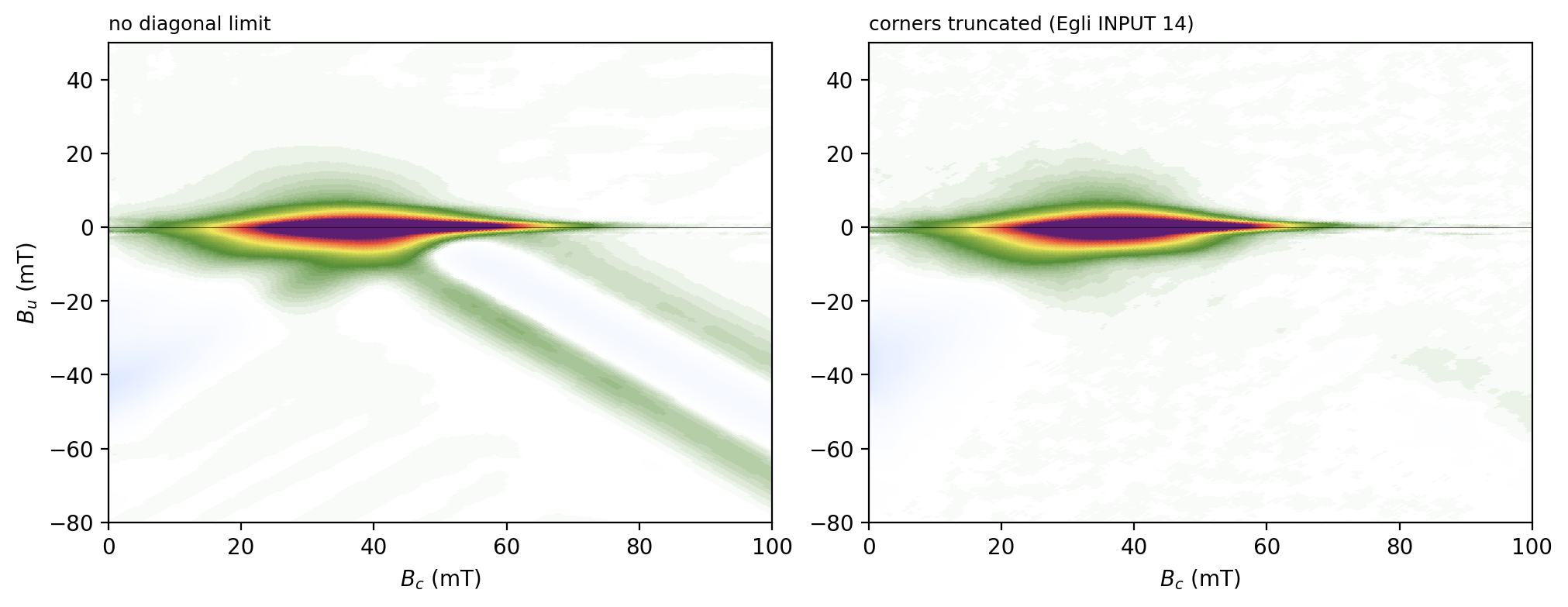
In the variforc_settings interface the same thing is requested with a single
diagonal_limit argument, which places the truncation automatically at the coercive field
estimated from the measurements.
7. Fidelity to the published algorithm
The implementation here is independent: it was written from the equations in Egli (2013) and the parameter semantics documented in the VARIFORC manual, not from the VARIFORC source, which is separately licensed.
The strongest available check is one Egli states quantitatively. His Eq. 7 defines a
synthetic magnetization surface, M = -4|B_u|, that is not physical but produces the
unit ridge ρ = δ(Bu) exactly. His Eq. 9 then predicts the width of that ridge
after processing: ΔHb = (1.076 sb − 0.468) δH. Reproducing that
relation without having been fitted to it tests the weight function, the rectangle
geometry and the coefficient extraction together.
dH = 0.001
Ha_r = np.arange(-0.20, 0.05 + dH / 2, dH)
Hb_r = np.arange(-0.20, 0.20 + dH / 2, dH)
A, B = np.meshgrid(Ha_r, Hb_r, indexing='ij')
ideal = -4.0 * np.abs(0.5 * (B + A))
ideal[B < A] = np.nan
Bu_r, Bc_r = forc.bu_bc_from_ha_hb(Ha_r, Hb_r)

print(f"{'s_b':>5} {'measured FWHM/dH':>18} {'Egli Eq. 9':>12} {'difference':>12}")
for sb in (2.0, 3.0, 5.0, 8.0, 10.0):
    rho = forc.variforc_rho_from_grid(Ha_r, Hb_r, ideal, sc0=6, sc1=6,
                                      sb0=sb, sb1=sb, lambda_c=0.0,
                                      lambda_b=0.0, dH=dH, min_pts=8)
    band = (Bc_r > 0.04) & (Bc_r < 0.06) & (np.abs(Bu_r) < 0.03) & np.isfinite(rho)
    centres, profile = forc.bin_profile(Bu_r[band], rho[band], -0.03, 0.03,
                                        n_bins=240)
    measured = forc.profile_peak_and_fwhm(centres, profile,
                                          use_abs=False)['fwhm'] / dH
    predicted = 1.076 * sb - 0.468
    print(f"{sb:5.1f} {measured:18.3f} {predicted:12.3f} "
          f"{100 * (measured - predicted) / predicted:11.1f}%")
s_b measured FWHM/dH Egli Eq. 9 difference
2.0 1.678 1.684 -0.4%
3.0 2.746 2.760 -0.5%
5.0 4.898 4.912 -0.3%
  8.0              8.134        8.140        -0.1%
 10.0             10.295       10.292         0.0%
The measured relation is within about half a percent of the published one across the range. Alongside this, the test suite checks the estimator against an analytic quadratic surface (agreeing with the independent mixed-derivative estimator to 5 × 10⁻¹¹), against a Preisach assemblage with a closed-form distribution, and confirms that the propagated uncertainty matches the scatter of ρ over independent noise realizations.
Further detail, including the differences that remain from VARIFORC, is in
forc
Summary
Variable smoothing lets the regression window grow where the FORC function is genuinely smooth and holds it narrow across ridges, giving a sharper ridge and a quieter background than any single window achieves.
Describe the sample with
variforc_settingsand a preset; setsmoothing_factorandgrowth_rate, and report both with any diagram.Turn on
estimate_uncertaintyto see which parts of the diagram the data support. SNR3 is the conventional significance threshold.
Use a diagonal limit for samples with near-rectangular loops, where large windows would otherwise smear artefacts along the coercive-field diagonals.
Variable smoothing earns its cost on noisy data. On very clean measurements a well-chosen constant window does just as well.
References
Egli, R., Chen, A. P., Winklhofer, M., Kodama, K. P., & Horng, C.-S. (2010). Detection of noninteracting single domain particles using first-order reversal curve diagrams. Geochemistry, Geophysics, Geosystems, 11, Q01Z11. Egli et al. (2010)
Egli, R. (2013). VARIFORC: An optimized protocol for calculating non-regular first-order reversal curve (FORC) diagrams. Global and Planetary Change, 110, 302–320. Egli (2013)
Harrison, R. J., & Feinberg, J. M. (2008). FORCinel: An improved algorithm for calculating first-order reversal curve distributions using locally weighted regression smoothing. Geochemistry, Geophysics, Geosystems, 9, Q05016. Harrison & Feinberg (2008)
Heslop, D., & Roberts, A. P. (2012). Estimation of significance levels and confidence intervals for first-order reversal curve distributions. Geochemistry, Geophysics, Geosystems, 13, Q12Z40. Heslop & Roberts (2012)
Ludwig, P., Egli, R., Bishop, S., Chernenko, V., Frederichs, T., Rugel, G., Merchel, S., & Orgeira, M. J. (2013). Characterization of primary and secondary magnetite in marine sediment by combining chemical and magnetic unmixing techniques. Global and Planetary Change, 110, 321–339. Ludwig et al. (2013)
Pike, C. R., Roberts, A. P., & Verosub, K. L. (1999). Characterizing interactions in fine magnetic particle systems using first order reversal curves. Journal of Applied Physics, 85, 6660–6667. Pike et al. (1999)
- Egli, R. (2013). VARIFORC: An optimized protocol for calculating non-regular first-order reversal curve (FORC) diagrams. Global and Planetary Change, 110, 302–320. 10.1016/j.gloplacha.2013.08.003
- Heslop, D., & Roberts, A. P. (2012). Estimation of significance levels and confidence intervals for first‐order reversal curve distributions. Geochemistry, Geophysics, Geosystems, 13(5). 10.1029/2012gc004115
- Egli, R., Chen, A. P., Winklhofer, M., Kodama, K. P., & Horng, C. (2010). Detection of noninteracting single domain particles using first‐order reversal curve diagrams. Geochemistry, Geophysics, Geosystems, 11(1). 10.1029/2009gc002916
- Harrison, R. J., & Feinberg, J. M. (2008). FORCinel: An improved algorithm for calculating first‐order reversal curve distributions using locally weighted regression smoothing. Geochemistry, Geophysics, Geosystems, 9(5). 10.1029/2008gc001987
- Ludwig, P., Egli, R., Bishop, S., Chernenko, V., Frederichs, T., Rugel, G., Merchel, S., & Orgeira, M. J. (2013). Characterization of primary and secondary magnetite in marine sediment by combining chemical and magnetic unmixing techniques. Global and Planetary Change, 110, 321–339. 10.1016/j.gloplacha.2013.08.018
- Pike, C. R., Roberts, A. P., & Verosub, K. L. (1999). Characterizing interactions in fine magnetic particle systems using first order reversal curves. Journal of Applied Physics, 85(9), 6660–6667. 10.1063/1.370176