FORC Processing - RockmagPy Documentation

This notebook takes a first-order reversal curve measurement from the raw instrument file to a FORC distribution, plots profiles through it, and generates a MagIC measurements table. It starts with the workflow and then goes into more detail.

For what a FORC diagram represents and the field conventions used throughout, see the FORC introduction.

pmagpy.forc takes FORC data from a raw Lake Shore (Princeton MicroMag) VSM file, or from a MagIC measurements table, through to diagrams and quantitative profiles.

This notebook goes in this order:

The workflow: a FORC diagram, profiles, and a ridge-following profile.
The measurement and the distribution: what a FORC is and how ρ is estimated.
Reading raw instrument files: units, header tags, and segmentation.
Drift correction.
Archiving to MagIC, and reprocessing from a MagIC measurements table.
Choosing the smoothing level.
Relationship to FORCinel and VARIFORC.

Smoothing is developed much further in FORC_smoothing.ipynb, and the design and caveats of the implementation are collected in forc_implementation_notes.md.

Install and import packages¶

import numpy as np
import matplotlib.pyplot as plt

import pmagpy.forc as forc

%matplotlib inline
%config InlineBackend.figure_format = 'retina'

1. The workflow¶

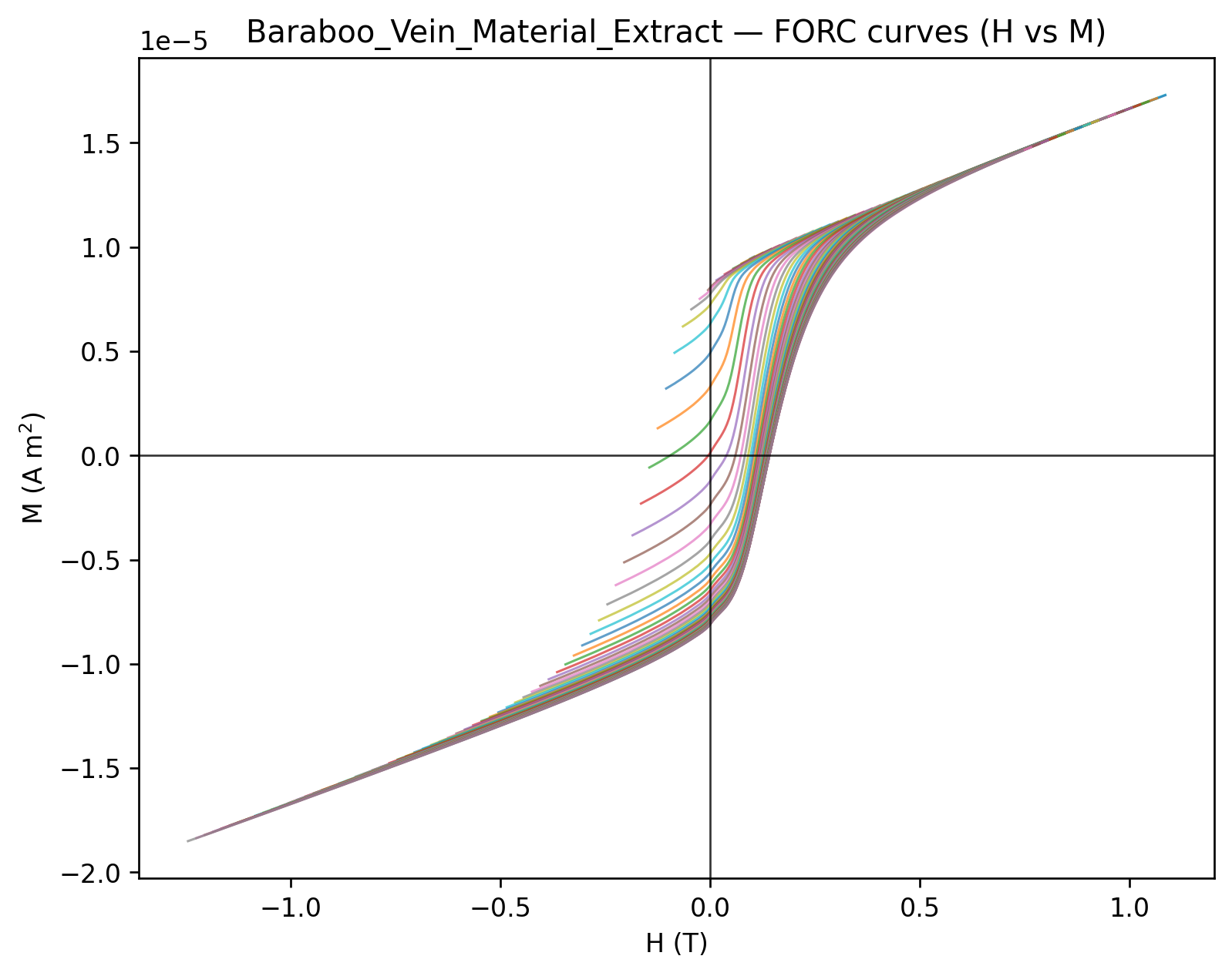
The example dataset is vein-hosted hematite measured on the Lake Shore 8600 VSM at the Institute for Rock Magnetism by Maxwell Brown: 269 reversal curves to 1.09 T, distributed with these notebooks both as the raw instrument file and as a MagIC measurements table.

process_forc reads the measurements, corrects instrument drift, estimates the FORC distribution with an automatically chosen smoothing level, and draws the diagram. mode selects the input: 'i' for one raw file, 'm' for a MagIC measurements table, 'b' to batch a directory, 's' to stack replicate runs.

out = forc.process_forc(
    mode='m',
    path='../example_data/FORC/baraboo_vein_MagIC/measurements.txt',
    do_regrid=True,          # put the curves on a common field lattice
    B_step=0.005,            # at the 5 mT measurement increment
    Bu_min=-0.15,            # plotted window, asymmetric because this
    Bu_max=0.075,            # distribution sits below the Bu = 0 axis
    Bc_max=0.6,
    color_scale_version=2,
    plot_fraction=0.25,      # show a quarter of the measured curves
    display_upsample_factor=2,
    verbose=False,
)

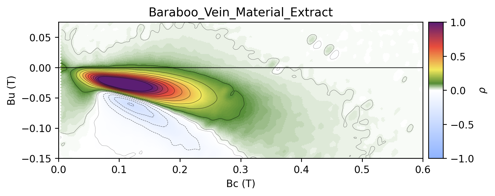
The distribution has a peak offset below the B_u = 0 axis, a coercivity distribution extending beyond 400 mT, and a negative region below the central peak. This combination has been documented for natural hematite (Roberts et al., 2006).

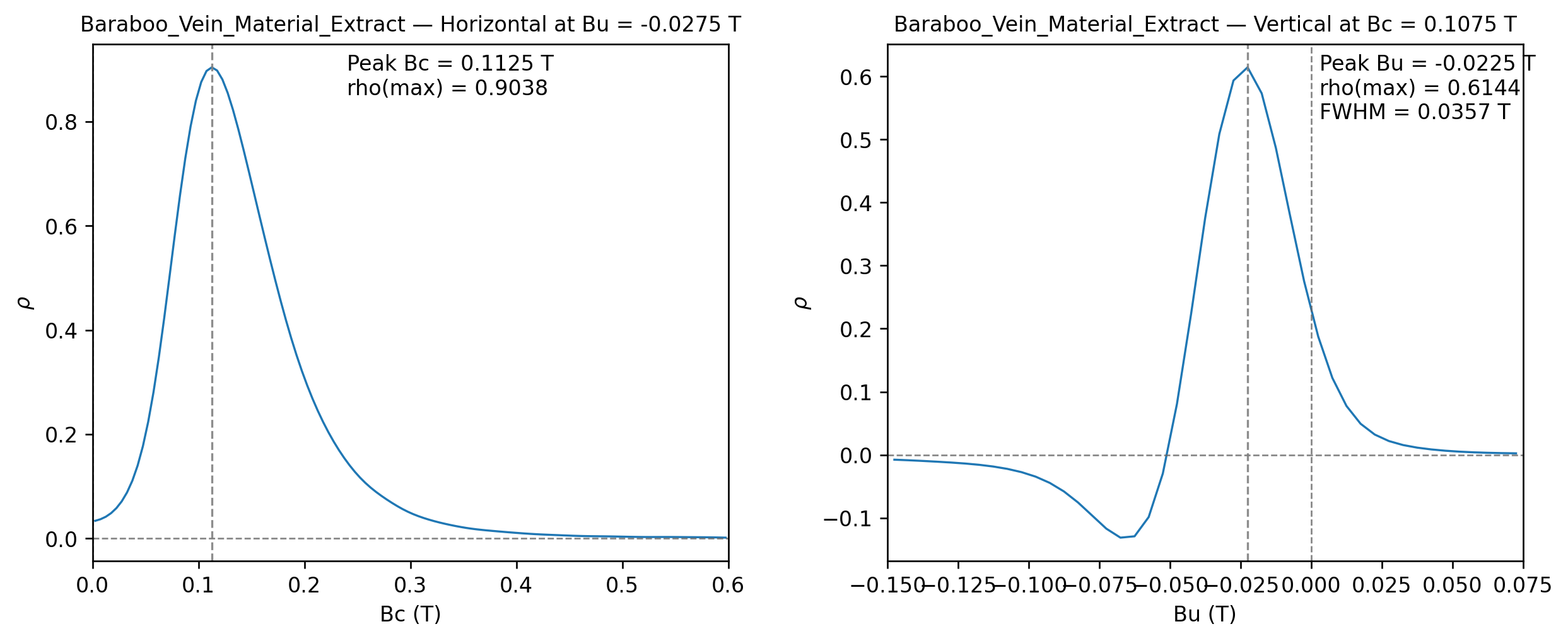
Profiles through the peak quantify these characteristics: ρ against B_c at the peak B_u, and ρ against B_u at the peak B_c, each with a peak position and width.

forc.plot_auto_forc_profiles(out, smooth_sigma_bins=2.5, export_txt=False,
                             export_png=False)

Peak rho point inside bounded plot area:
  Bu = -0.027500 T
  Bc = 0.107500 T
  rho = 1.000000

Additional smoothing is applied to the profiles, which changes the peak rho, Bc and Bu values:
  Peak Bu on profile = -0.022500 T
  Peak Bc on profile = 0.112500 T
  Bu-profile FWHM = 0.035725 T

A fixed-B_u cut assumes the crest of the distribution stays at one B_u. For this sample, that assumption does not hold: the crest drifts to more negative B_u as coercivity increases, so a horizontal cut through the peak comes off the ridge. The function ridge_profile shows values along the crest instead.

ridge = forc.ridge_profile(out['Ha_vals_used'], out['Hb_vals_used'], out['rho'],
                           Bu_min=-0.15, Bu_max=0.05, Bc_min=0.01, Bc_max=0.5)

peak = forc.find_bounded_peak_rho(out['Ha_vals_used'], out['Hb_vals_used'], out['rho'])
horizontal = forc.slice_profile_smoothed(
    out['Ha_vals_used'], out['Hb_vals_used'], out['rho'],
    mode='Bu', target=peak['bu'], x_min=0.0, x_max=0.6, bin_width=0.001,
    smooth_sigma_bins=2.5)

print(f"peak of the distribution : Bc = {1e3 * peak['bc']:.1f} mT, "
      f"Bu = {1e3 * peak['bu']:.1f} mT")
print(f"crest Bu range           : {1e3 * np.nanmin(ridge['bu']):.1f} to "
      f"{1e3 * np.nanmax(ridge['bu']):.1f} mT")
print(f"FWHM, fixed-Bu profile   : {1e3 * horizontal['peak']['fwhm']:.0f} mT")
print(f"FWHM, along the crest    : {1e3 * ridge['peak']['fwhm']:.0f} mT")

peak of the distribution : Bc = 107.5 mT, Bu = -27.5 mT
crest Bu range           : -97.6 to -2.6 mT
FWHM, fixed-Bu profile   : 103 mT
FWHM, along the crest    : 123 mT

fig, (ax_map, ax_prof) = plt.subplots(1, 2, figsize=(10, 3.8), constrained_layout=True)

Ha, Hb, rho = out['Ha_vals_used'], out['Hb_vals_used'], out['rho']
vmax = forc.rho_window_vmax(Ha, Hb, rho, pct=100, Bu_min=-0.15, Bu_max=0.075,
                             Bc_min=0.0, Bc_max=0.6)
Ha_e, Hb_e = np.meshgrid(forc.centers_to_edges(Ha),
                         forc.centers_to_edges(Hb), indexing='ij')
mesh = ax_map.pcolormesh(1e3 * 0.5 * (Hb_e - Ha_e), 1e3 * 0.5 * (Hb_e + Ha_e),
                         rho / vmax, cmap=forc.get_forc_cmap(2),
                         vmin=-1, vmax=1, shading='auto')
ax_map.plot(1e3 * ridge['bc'], 1e3 * ridge['bu'], 'k-', lw=1.4, label='tracked crest')
ax_map.axhline(1e3 * peak['bu'], color='#0072B2', lw=0.9, ls=(0, (4, 3)),
               label=r'fixed $B_u$ cut')
ax_map.axhline(0, color='k', lw=0.5, alpha=0.6)
ax_map.set_xlim(0, 500)
ax_map.set_ylim(-150, 75)
ax_map.set_xlabel(r'$B_c$ (mT)')
ax_map.set_ylabel(r'$B_u$ (mT)')
ax_map.legend(fontsize=8, loc='upper right')
fig.colorbar(mesh, ax=ax_map, label=r'$\rho\,/\,\rho_{max}$', fraction=0.046)

ax_prof.plot(1e3 * horizontal['x'], horizontal['y'] / vmax, color='#0072B2',
             lw=1.0, ls=(0, (4, 3)), label=r'fixed $B_u$ profile')
ax_prof.plot(1e3 * ridge['bc'], ridge['rho'] / vmax, 'k-', lw=1.4,
             label='ridge-following profile')
ax_prof.axhline(0, color='0.85', lw=0.6)
ax_prof.set_xlim(0, 500)
ax_prof.set_xlabel(r'$B_c$ (mT)')
ax_prof.set_ylabel(r'$\rho\,/\,\rho_{max}$')
ax_prof.legend(frameon=False, fontsize=8)
plt.show()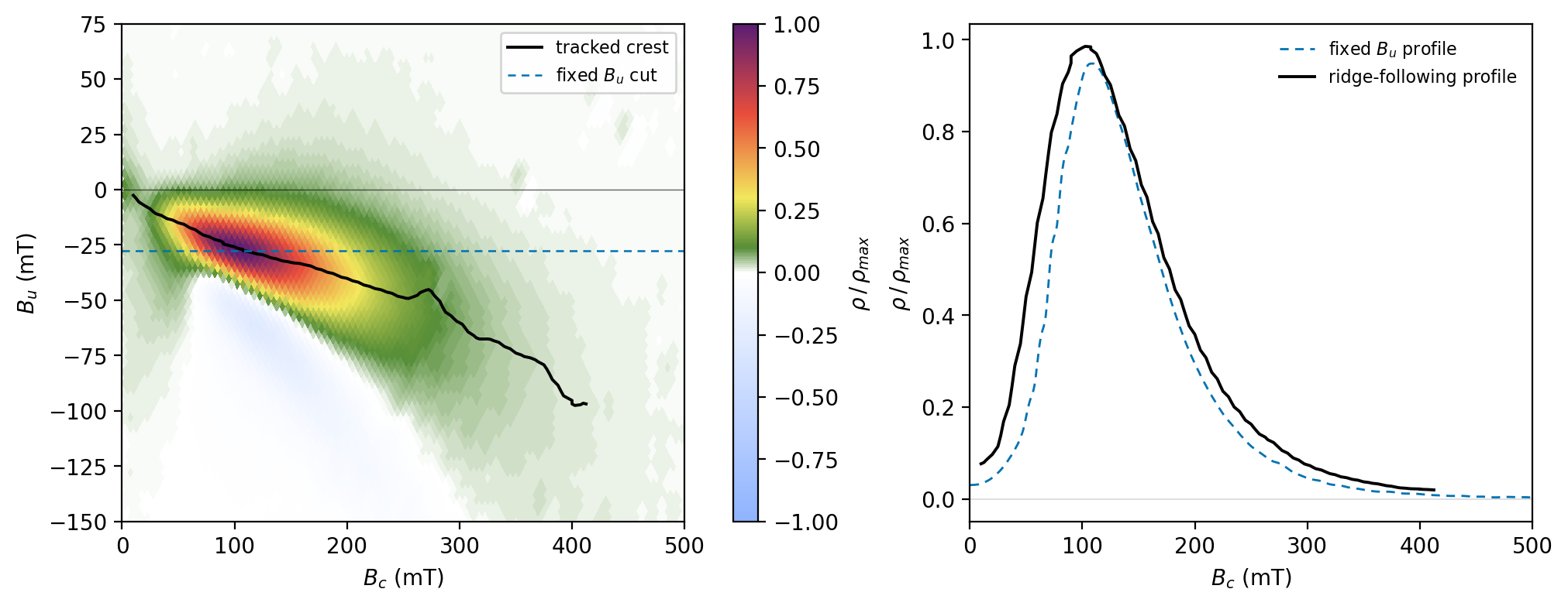

The ridge-following profile recovers amplitude on the high-coercivity limb that the fixed-B_u cut misses.

Each processing decision is recorded in the returned dictionary, so a diagram can be reported together with the choices that produced it.

loess = out['loess_params']
print(f"calibration points : {out['n_calibration_points']}")
print(f"drift correction   : {out['drift_corrected']} ({out['drift_fit']})")
print(f"grid               : {out['rho'].shape[0]} reversal x "
      f"{out['rho'].shape[1]} applied fields, {1e3 * out['dHa_used']:.0f} mT steps")
print(f"LOESS spans        : {1e3 * loess['span_Ha_T_used']:.0f} mT x "
      f"{1e3 * loess['span_Hb_T_used']:.0f} mT, min_pts = {loess['min_pts_used']}")

calibration points : 270
drift correction   : True (linear)
grid               : 268 reversal x 468 applied fields, 5 mT steps
LOESS spans        : 25 mT x 25 mT, min_pts = 34

2. The marginal coercivity distribution¶

Integrating ρ along the interaction-field axis at each coercivity collapses the diagram to one dimension,

f(B_c) = \int \rho(B_c, B_u)\, dB_u,

(1)

which is the coercivity distribution the assemblage would show in the absence of interactions. It is directly comparable to a coercivity distribution obtained by differentiating a backfield demagnetization curve, and to the components recovered by unmixing (see coercivity_unmixing.ipynb), so it provides a bridge between FORC analysis and the more widely applied coercivity-spectrum methods.

Two things are worth keeping in mind. The integral runs over the $B_u$ window given, so a window that clips the tails of an offset distribution — as a hematite distribution centred well below $B_u = 0$ would be — will underestimate $f$ . And because the integration averages along $B_u$ , the result is much less sensitive to the smoothing level than the two-dimensional diagram is.

cdist = forc.coercivity_distribution(
    out['Ha_vals_used'], out['Hb_vals_used'], out['rho'],
    Bu_min=-0.30, Bu_max=0.15, Bc_max=0.60, smooth_sigma_bins=2.0,
)

fig, (ax_map, ax_cd) = plt.subplots(1, 2, figsize=(10.5, 3.8),
                                    constrained_layout=True)

# the diagram, with the integration window marked
Ha, Hb, rho = out['Ha_vals_used'], out['Hb_vals_used'], out['rho']
vmax = forc.rho_window_vmax(Ha, Hb, rho, pct=100, Bu_min=-0.15, Bu_max=0.075,
                             Bc_min=0.0, Bc_max=0.6)
Ha_e, Hb_e = np.meshgrid(forc.centers_to_edges(Ha),
                         forc.centers_to_edges(Hb), indexing='ij')
ax_map.pcolormesh(1e3 * 0.5 * (Hb_e - Ha_e), 1e3 * 0.5 * (Hb_e + Ha_e), rho / vmax,
                  cmap=forc.get_forc_cmap(2), vmin=-1, vmax=1, shading='auto')
ax_map.axhline(-300, color='0.2', lw=0.9, ls='--')
ax_map.axhline(150, color='0.2', lw=0.9, ls='--')
ax_map.set_xlim(0, 600)
ax_map.set_ylim(-320, 170)
ax_map.set_xlabel(r'$B_c$ (mT)')
ax_map.set_ylabel(r'$B_u$ (mT)')
ax_map.set_title('integrate between the dashed lines', fontsize=9, loc='left')

forc.plot_coercivity_distribution(cdist, ax=ax_cd)
plt.show()

print(f"peak    {1e3 * cdist['peak']['peak_x']:.0f} mT")
print(f"FWHM    {1e3 * cdist['peak']['fwhm']:.0f} mT")

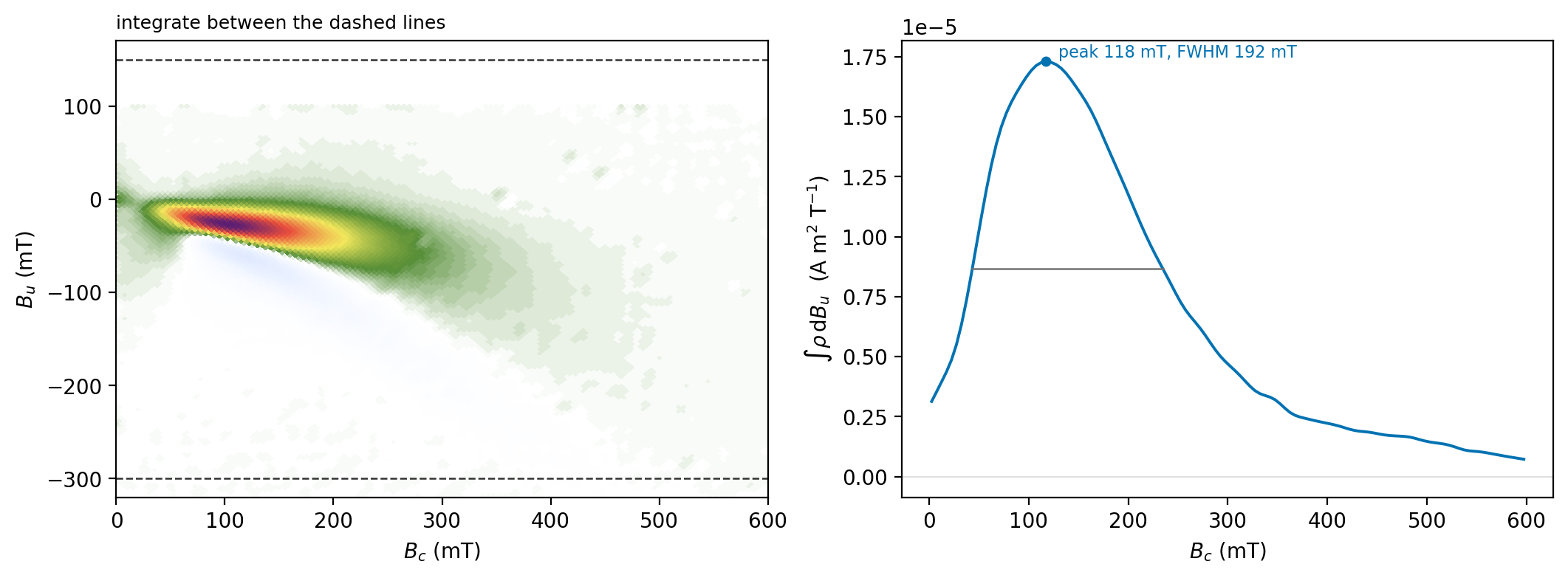
peak    118 mT
FWHM    192 mT

The marginal peak at 118 mT sits close to the 108 mT peak of the two-dimensional diagram. The width is different: 192 mT here against 103 mT for the fixed- $B_u$ horizontal profile and 123 mT along the tracked crest. A cut samples one line through the distribution, whereas this integrates every line, so it picks up the coercivity spread carried by the parts of the distribution that lie away from the crest.

That is the standard workflow. The rest of the notebook explains what those calls did and where the choices matter.

3. The measurement and the distribution¶

A FORC is a partial hysteresis curve that samples the interior of the major loop (Pike et al., 1999). Each curve is measured by applying a positive saturating field, decreasing the field along the descending branch of the major loop to a reversal field $H_a$ , and then measuring the magnetization $M$ at increasing field steps as the field is returned from $H_a$ to the maximum field. The field at which each measurement is made is the applied field $H_b$ , and by construction $H_b \geq H_a$ .

Repeating this for successively lower reversal fields, resaturating before each curve, fills the region enclosed by the major loop and defines the magnetization surface $M(H_a, H_b)$ on the half-plane $H_b \geq H_a$ . The FORC distribution is its mixed second derivative,

\rho(H_a, H_b) = -\frac{1}{2}\,\frac{\partial^2 M(H_a, H_b)}{\partial H_a \, \partial H_b},

(2)

conventionally displayed in the rotated coordinates

B_c = \frac{H_b - H_a}{2}, \qquad B_u = \frac{H_b + H_a}{2},

(3)

with $B_c$ a coercivity axis and $B_u$ an interaction or bias axis.

Because ρ is a second derivative of measured data, it cannot be estimated without smoothing. pmagpy.forc fits a weighted local quadratic surface (LOESS with tricube weights) over an elliptical neighbourhood of each grid node and reads ρ off the mixed-derivative coefficient. The size of that neighbourhood is the LOESS span, and it is the one consequential analytical choice in FORC processing.

pmagpy.forc uses these symbols with the meanings above, matching Pike et al. (1999), Roberts et al. (2000), Harrison and Feinberg (2008) and Egli (2013). Fields are handled in tesla and moments in A m² throughout.

One naming collision is worth flagging: MicroMag file headers use Hb1/Hb2 for the bias axis limits of the FORC diagram and Hc1/Hc2 for the coercivity axis limits. Those are display bounds, unrelated to the reversal and applied fields. pmagpy.forc reads them into Bu_max and Bc_max.

4. Reading raw instrument files¶

The workflow above started from the MagIC table. Starting from the raw instrument file is a one-argument change (mode='i'), but it is worth seeing what the reader works out.

MicroMag writes either SI or cgs depending on an instrument setting, and older exports default to cgs. Reading Oe as tesla would introduce a silent factor of 10⁴, so the units are resolved explicitly and the converted field range is range-checked.

raw_file = '../example_data/FORC/baraboo_vein_material_hematite.txt'

units = forc.read_file_units(raw_file)
print(f"field in {units['field_unit']}, moment in {units['moment_unit']} "
      f"(determined from the {units['source']})")

tags, data_start = forc.read_header_tags_and_data_start(raw_file)
for name in ['HCal', 'HSat', 'Hb1', 'Hb2', 'Hc1', 'Hc2', 'NForc']:
    if name in tags:
        print(f"  {name:6s} {tags[name]:g}")

field in T, moment in A m^2 (determined from the units line)
  HCal   1.1
  HSat   1.8
  Hb1    -0.25
  Hb2    0.1
  Hc2    1
  NForc  270

Header tags are reported in tesla after conversion. HCal is the field at which the calibration measurements are made, HSat the saturating field applied before each curve.

The numeric section is then split into calibration points and reversal curves. Rows may carry a third column (temperature on some exports), and blocks may be separated by blank lines, by a large downward jump in field, or by the calibration-point pattern.

segments, _ = forc.phase1_prepare_segments_dual(raw_file, export_magic=False)

cal = [s for s in segments if s.kind == 'cal']
curves = [s for s in segments if s.kind == 'forc']
print(f"\n{len(cal)} calibration points, {len(curves)} reversal curves")
print(f"reversal fields Ha span {min(s.Ha for s in curves):+.3f} to "
      f"{max(s.Ha for s in curves):+.3f} T")

Parsed 269 curve blocks and 270 calibration points | curve length min/median/max = 3/271/399
Drift correction (linear) from 270 calibration points: +1.321e-08 A m^2 over the run

270 calibration points, 269 reversal curves
reversal fields Ha span -1.245 to +0.095 T

5. Drift correction¶

A calibration measurement is made at a fixed field before every reversal curve. Any change in the measured moment at that field over the run is instrument drift, and it is removed by interpolating the calibration record across the measurement sequence.

If fewer than two calibration points are identified the pipeline says so explicitly rather than silently returning uncorrected curves, and out['drift_corrected'] records what happened.

segments_raw = forc.read_segments_raw(raw_file, HCal=float(tags['HCal']), verbose=False)
segments_raw = forc.split_cal_first_point(segments_raw, HCal=float(tags['HCal']))
drift, cal_pos, cal_M = forc.compute_drift_from_cals(segments_raw, fit='linear')

fig, ax = plt.subplots(figsize=(6, 3.2), constrained_layout=True)
ax.plot(np.arange(cal_M.size), 1e9 * (cal_M - cal_M[0]), '.', ms=3, color='#0072B2')
ax.set_xlabel('calibration point number')
ax.set_ylabel('drift (nAm$^2$)')
ax.set_title(f'total drift {1e9 * (cal_M[-1] - cal_M[0]):+.2f} nAm$^2$, '
             f'{100 * (cal_M[-1] - cal_M[0]) / cal_M[0]:+.2f}% of the calibration moment',
             fontsize=9, loc='left')
plt.show()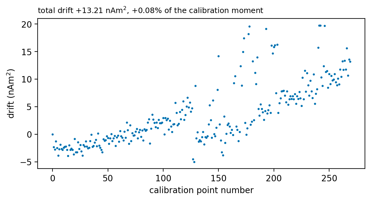

The drift here is small but systematic, and removing it is cheap; for this specimen it changes ρ by at most about 1% of the distribution maximum. drift_fit='pchip' uses a monotone piecewise-cubic interpolation when the drift is not linear.

6. Archiving to MagIC¶

A published FORC diagram cannot be re-smoothed or reprocessed from the figure alone, and FORC data have rarely been archived at the measurement level. export_magic_measurements_from_raw writes each field–moment pair as a row of a MagIC measurements table under the LP-FORC method code, including the calibration measurements, so the drift correction remains reproducible from the archive.

magic_file = forc.export_magic_measurements_from_raw(
    raw_file,
    out_dir='../example_data/FORC/baraboo_vein_MagIC',
    filename='measurements.txt',
    specimen='Baraboo_Vein_Material_Extract',
    experiment='IRM_VSM_Lake_Shore-LP-FORC-251142',
    instrument_codes='IRM_VSM_Lake_Shore',
    meas_temp_k=294,
    citations='This study',
)
print(f'wrote {magic_file}')

wrote ../example_data/FORC/baraboo_vein_MagIC/measurements.txt

The result is a standard MagIC measurements table, readable with the same tools used throughout these notebooks.

import pmagpy.contribution_builder as cb

contribution = cb.Contribution('../example_data/FORC/baraboo_vein_MagIC')
measurements = contribution.tables['measurements'].df
print(f"{len(measurements)} measurements, "
      f"method codes {list(measurements['method_codes'].unique())}")
measurements[['measurement', 'specimen', 'meas_field_dc', 'magn_moment']].head()

-I- Using online data model

-I- Getting method codes from earthref.org

-I- Importing controlled vocabularies from https://earthref.org

68200 measurements, method codes ['LP-FORC']

The point of archiving the measurements is that nothing is lost. Processing the raw instrument file directly and processing the MagIC table give the same distribution.

out_raw = forc.process_forc(
    mode='i', path=raw_file, do_regrid=True, B_step=0.005,
    plot_hyst=False, plot_rho=False, verbose=False,
)

shared = np.isfinite(out['rho']) & np.isfinite(out_raw['rho'])
difference = np.max(np.abs(out['rho'][shared] - out_raw['rho'][shared]))
print(f"shared grid cells        : {shared.sum()}")
print(f"max |rho_MagIC - rho_raw|: {difference:.3e} "
      f"({difference / np.nanmax(np.abs(out_raw['rho'])):.1e} of the maximum)")

shared grid cells        : 67662
max |rho_MagIC - rho_raw|: 0.000e+00 (0.0e+00 of the maximum)

7. Choosing the smoothing level¶

Double differentiation amplifies measurement noise, so some smoothing is unavoidable, and how much is applied changes the result. guess_loess_params sets a starting point from the geometry of the measurement rather than from the data values, and smooth_strength scales it. The figure below shows the same data across a factor of six in window size.

strengths = [0.5, 1.0, 2.0, 3.0]
fig, axes = plt.subplots(1, len(strengths), figsize=(13, 3.4),
                         constrained_layout=True, sharey=True)

for ax, strength in zip(axes, strengths):
    trial = forc.process_forc(
        mode='i', path=raw_file, do_regrid=True, B_step=0.005,
        smooth_strength=strength, plot_hyst=False, plot_rho=False, verbose=False,
    )
    Ha, Hb, rho = trial['Ha_vals_used'], trial['Hb_vals_used'], trial['rho']
    vmax = forc.rho_window_vmax(Ha, Hb, rho, pct=100, Bu_min=-0.15, Bu_max=0.075,
                                 Bc_min=0.0, Bc_max=0.6)
    Ha_e, Hb_e = np.meshgrid(forc.centers_to_edges(Ha),
                             forc.centers_to_edges(Hb), indexing='ij')
    ax.pcolormesh(1e3 * 0.5 * (Hb_e - Ha_e), 1e3 * 0.5 * (Hb_e + Ha_e), rho / vmax,
                  cmap=forc.get_forc_cmap(2), vmin=-1, vmax=1, shading='auto')
    ax.set_xlim(0, 400)
    ax.set_ylim(-150, 75)
    ax.set_xlabel(r'$B_c$ (mT)')
    span = 1e3 * trial['loess_params']['span_Ha_T_used']
    ax.set_title(f'smooth_strength = {strength}\nspan = {span:.0f} mT',
                 fontsize=9, loc='left')

axes[0].set_ylabel(r'$B_u$ (mT)')
plt.show()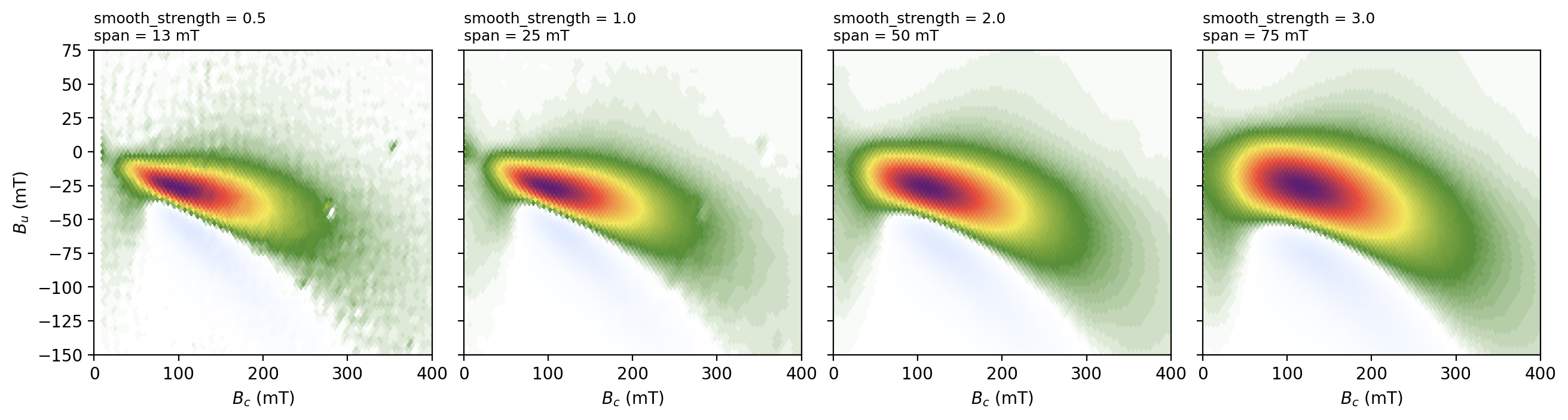

The peak position is stable across this range; its width is not. Report the spans in out['loess_params'] with any diagram.

FORC_smoothing.ipynb develops this: what the neighbourhood is, how much of it is usable near the B_c = 0 axis, what over- and under-smoothing do to a feature of known width, a residual-based criterion for choosing a level, and why a single window cannot serve a narrow ridge and a broad background at once.

A note on profile binning¶

Profiles are binned at the grid step over the requested window. This matters here: the lowest reversal curves reach -1.245 T, so a fixed number of bins spread over the full measured range would be far coarser than the plotted window and would quantize the reported peak position. smooth_sigma_bins is a Gaussian sigma in bins, so its physical width scales with the bin width. plot_custom_forc_profiles takes user-chosen B_u and B_c values rather than the peak, for interrogating a shoulder or a secondary feature.

8. Relationship to other FORC packages¶

The processing lineage of FORC analysis is largely a lineage of smoothing strategies, and it is worth being explicit about where pmagpy.forc sits relative to the packages in widest use.

	Roberts et al. (2000)	FORCinel	VARIFORC	FORCsensei	`pmagpy.forc`
smoothing	polynomial over a square neighbourhood, integer smoothing factor	LOESS, tricube weights	LOESS with spatially variable smoothing factors	constant and VARIFORC-style variable smoothing	LOESS tricube, or VARIFORC-style variable smoothing
smoothing selection	user	residual-based optimum smoothing factor	user-set factors with limits along $B_c$ , $B_b$ and the diagonals	Bayesian model selection over a parameter grid	automated from measurement geometry, scaled by `smooth_strength`; VARIFORC presets
variable smoothing	no	yes (VARIFORC implemented)	yes	yes	yes
uncertainty on ρ	no	no	error matrix, signal-to-noise threshold, confidence intervals	full posterior over smoothing models	propagated standard error and signal-to-noise ratio per cell
central-ridge isolation	no	yes (`IsolateCR`)	yes	no	no
marginal coercivity distribution	no	yes	yes	no	yes
$B_c$ ≈ 0 behaviour	truncated	constant smoothing maintained to the axis	explicit lower-diagonal trim factor	as VARIFORC	half-window near the diagonal; optional `edge_mask_bc_bins`
output grid	measurement grid	measurement grid	independent output mesh	measurement grid	measurement grid, optional regridding
MagIC read/write	no	no	no	no	yes
platform	—	Igor Pro (commercial)	Mathematica (commercial)	Python, MIT	Python, open source

The variable-smoothing kernel was written from the equations of Egli (2013) rather than from any existing code, and it is checked in two independent ways. It reproduces Egli’s published resolution law (his Eq. 9) for the processed width of a synthetic ridge, and it agrees with FORCsensei — an independently written implementation of the same protocol — to within 1 × 10^-11 of the peak amplitude on both case-study datasets distributed with that package, under constant and variable smoothing alike. That is the level of floating-point accumulation order. FORC_variforc.ipynb shows these comparisons.

Two gaps remain relative to FORCinel. pmagpy.forc does not implement central-ridge isolation or the mean-field correction, and it computes the distribution on the measurement grid rather than on an independent output mesh — VARIFORC’s decoupled mesh allows datasets measured with different protocols to be combined without interpolation.

What pmagpy.forc adds is not a new estimator but integration: the same processing sits in the Python environment where the rest of a rock magnetic workflow is carried out, its parameters are recorded in the output rather than in a session, and it reads and writes the MagIC data model directly — a fully scriptable path from the raw instrument file through an archived measurements table to a reproducible diagram.

Summary¶

process_forc takes a raw MicroMag file or a MagIC measurements table to a finished diagram in one call; mode selects individual, batch, stacked, or MagIC input.
Units are resolved from the file rather than assumed, and a file whose declared units are inconsistent with its data is rejected rather than silently rescaled.
Drift is corrected from the interleaved calibration measurements, and the pipeline reports when it could not be.
Export the measurements to MagIC (export_magic_measurements_from_raw). The archived table reproduces the distribution exactly, calibration points included.
The smoothing level is the consequential choice. Assess results across a range of smooth_strength and report the spans in out['loess_params'] with any diagram.
Use ridge_profile rather than a fixed-B_u cut where the crest of the distribution drifts with coercivity.
coercivity_distribution collapses ρ along B_u to a one-dimensional coercivity distribution comparable with backfield-derived spectra.

References¶

Egli, R. (2013). VARIFORC: An optimized protocol for calculating non-regular first-order reversal curve (FORC) diagrams. Global and Planetary Change, 110, 302–320. Egli (2013)
Harrison, R. J., & Feinberg, J. M. (2008). FORCinel: An improved algorithm for calculating first-order reversal curve distributions using locally weighted regression smoothing. Geochemistry, Geophysics, Geosystems, 9, Q05016. Harrison & Feinberg (2008)
Pike, C. R., Roberts, A. P., & Verosub, K. L. (1999). Characterizing interactions in fine magnetic particle systems using first order reversal curves. Journal of Applied Physics, 85, 6660–6667. Pike et al. (1999)
Roberts, A. P., Pike, C. R., & Verosub, K. L. (2000). First-order reversal curve diagrams: A new tool for characterizing the magnetic properties of natural samples. Journal of Geophysical Research, 105, 28461–28475. Roberts et al. (2000)
Roberts, A. P., Liu, Q., Rowan, C. J., Chang, L., Carvallo, C., Torrent, J., & Horng, C.-S. (2006). Characterization of hematite (α-Fe₂O₃), goethite (α-FeOOH), greigite (Fe₃S₄), and pyrrhotite (Fe₇S₈) using first-order reversal curve diagrams. Journal of Geophysical Research, 111, B12S35. Roberts et al. (2006)
Roberts, A. P., Heslop, D., Zhao, X., & Pike, C. R. (2014). Understanding fine magnetic particle systems through use of first-order reversal curve diagrams. Reviews of Geophysics, 52, 557–602. Roberts et al. (2014)
Heslop, D., & Roberts, A. P. (2012). Estimation of significance levels and confidence intervals for first-order reversal curve distributions. Geochemistry, Geophysics, Geosystems, 13, Q12Z40. Heslop & Roberts (2012)
Heslop, D., Roberts, A. P., Oda, H., Zhao, X., Harrison, R. J., Muxworthy, A. R., Hu, P.-X., & Sato, T. (2020). An automatic model selection-based machine learning framework to estimate FORC distributions. Journal of Geophysical Research: Solid Earth, 125, e2020JB020418. Heslop et al. (2020)

References¶

Roberts, A. P., Liu, Q., Rowan, C. J., Chang, L., Carvallo, C., Torrent, J., & Horng, C. (2006). Characterization of hematite (α‐Fe2O3), goethite (α‐FeOOH), greigite (Fe3S4), and pyrrhotite (Fe7S8) using first‐order reversal curve diagrams. Journal of Geophysical Research: Solid Earth, 111(B12). 10.1029/2006jb004715
Pike, C. R., Roberts, A. P., & Verosub, K. L. (1999). Characterizing interactions in fine magnetic particle systems using first order reversal curves. Journal of Applied Physics, 85(9), 6660–6667. 10.1063/1.370176
Harrison, R. J., & Feinberg, J. M. (2008). FORCinel: An improved algorithm for calculating first‐order reversal curve distributions using locally weighted regression smoothing. Geochemistry, Geophysics, Geosystems, 9(5). 10.1029/2008gc001987
Egli, R. (2013). VARIFORC: An optimized protocol for calculating non-regular first-order reversal curve (FORC) diagrams. Global and Planetary Change, 110, 302–320. 10.1016/j.gloplacha.2013.08.003
Roberts, A. P., Pike, C. R., & Verosub, K. L. (2000). First‐order reversal curve diagrams: A new tool for characterizing the magnetic properties of natural samples. Journal of Geophysical Research: Solid Earth, 105(B12), 28461–28475. 10.1029/2000jb900326
Roberts, A. P., Heslop, D., Zhao, X., & Pike, C. R. (2014). Understanding fine magnetic particle systems through use of first-order reversal curve diagrams: FORC diagrams. Reviews of Geophysics, 52(4), 557–602. 10.1002/2014rg000462
Heslop, D., & Roberts, A. P. (2012). Estimation of significance levels and confidence intervals for first‐order reversal curve distributions. Geochemistry, Geophysics, Geosystems, 13(5). 10.1029/2012gc004115
Heslop, D., Roberts, A. P., Oda, H., Zhao, X., Harrison, R. J., Muxworthy, A. R., Hu, P. ‐X., & Sato, T. (2020). An Automatic Model Selection‐Based Machine Learning Framework to Estimate FORC Distributions. Journal of Geophysical Research: Solid Earth, 125(10). 10.1029/2020jb020418