This notebook visualizes data from low-temperature experiments conducted on a Magnetic Property Measurement System (MPMS) instrument and exported to MagIC format. The measurements visualized here are considered direct current (DC) measurements of magnetic remanence, in contrast to the alternating current (AC) susceptibility measurements that are visualized in the MPMS_plot_ac.ipynb notebook.
In the following example, specimens from samples of diabase dikes from the East Central Minnesota batholith have undergone the following experiments:
RTSIRM (room-temperature saturation isothermal remanent magnetization): in this experiment, a pulsed field was applied at room temperature (300 K) to impart a saturation isothermal remanent magnetization (SIRM) with the specimen then being cycled down to 10 K (-263.15ºC) and back to room temperature. Typically, the magnetic remanence is measured during both the cooling and warming phases.
FC LTSIRM (field-cooled low-temperature saturation isothermal remanent magnetization): in this experiment, the specimens were cooled down to 10 K in the presence of a strong field and then warmed back up to room temperature. Typically, the magnetic remanence is measured during the warming phase.
ZFC LTSIRM (zero-field-cooled low-temperature saturation isothermal remanent magnetization): in this experiment, the specimens were cooled down to 10 K in a zero-field environment, pulsed with a strong field at 10 K, and then warmed back up to room temperature. Typically, the magnetic remanence is measured during the warming phase.
Import scientific python libraries
Run the cell below to import the functions needed for the notebook.
import pmagpy.rockmag as rmag
import pmagpy.contribution_builder as cb
import pmagpy.ipmag as ipmag

from bokeh.io import output_notebook
output_notebook(hide_banner=True)
%config InlineBackend.figure_format = 'retina'
-W- cartopy is not installed
If you want to make maps, install using conda:
conda install cartopy
Import data
We can take the same approach as in the rockmag_data_unpack.ipynb notebook to bring the MagIC data into the notebook as a Contribution. To bring in a different contribution, set the directory path (currently './example_data/ECMB') and the name of the file (currently 'magic_contribution_20213.txt') to be those relevant to your data.
# set the dir_path to the directory where the measurements.txt file is located
dir_path = '../example_data/ECMB'

# set the name of the MagIC file
ipmag.unpack_magic('magic_contribution_20213.txt',
                     dir_path = dir_path,
                     input_dir_path = dir_path,
                     print_progress=False)

# create a contribution object from the tables in the directory
contribution = cb.Contribution(dir_path)
measurements = contribution.tables['measurements'].df
1 records written to file /Users/penokean/0000_GitHub/RockmagPy-notebooks/example_data/ECMB/contribution.txt
1 records written to file /Users/penokean/0000_GitHub/RockmagPy-notebooks/example_data/ECMB/locations.txt
90 records written to file /Users/penokean/0000_GitHub/RockmagPy-notebooks/example_data/ECMB/sites.txt
312 records written to file /Users/penokean/0000_GitHub/RockmagPy-notebooks/example_data/ECMB/samples.txt
1574 records written to file /Users/penokean/0000_GitHub/RockmagPy-notebooks/example_data/ECMB/specimens.txt
17428 records written to file /Users/penokean/0000_GitHub/RockmagPy-notebooks/example_data/ECMB/measurements.txt
-I- Using online data model
-I- Getting method codes from earthref.org
-I- Importing controlled vocabularies from https://earthref.org
Plot data
We can now plot the MPMS data within the measurements file using the rmag.plot_mpms_dc_interactive() function.
rmag.plot_mpms_dc_interactive(measurements)Extract MPMS data for a single specimen
We can now extract the MPMS data for a specific specimen.
First, we need to define the specimen for which we are extracting the data. To do this, we set specimen_name to be equal to a string (i.e. the specimen name within quotation marks).
Then, we can apply the rmag.extract_mpms_data_dc function to extract the data for that specimen.
specimen_name = 'NED4-1c'
fc_data, zfc_data, rtsirm_cool_data, rtsirm_warm_data = rmag.extract_mpms_data_dc(measurements, specimen_name)
Plot the data for a single specimen
rmag.plot_mpms_dc(fc_data, zfc_data, rtsirm_cool_data, rtsirm_warm_data)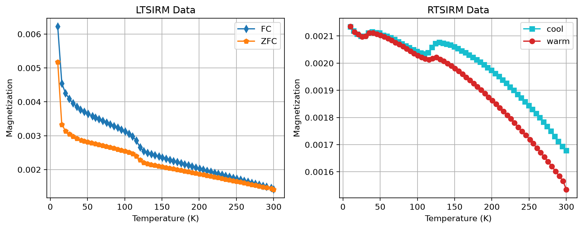
Plot the derivative
By setting plot_derivative=True, the derivative of the experimental data will be calculated and plotted.
rmag.plot_mpms_dc(fc_data, zfc_data, rtsirm_cool_data, rtsirm_warm_data, plot_derivative=True)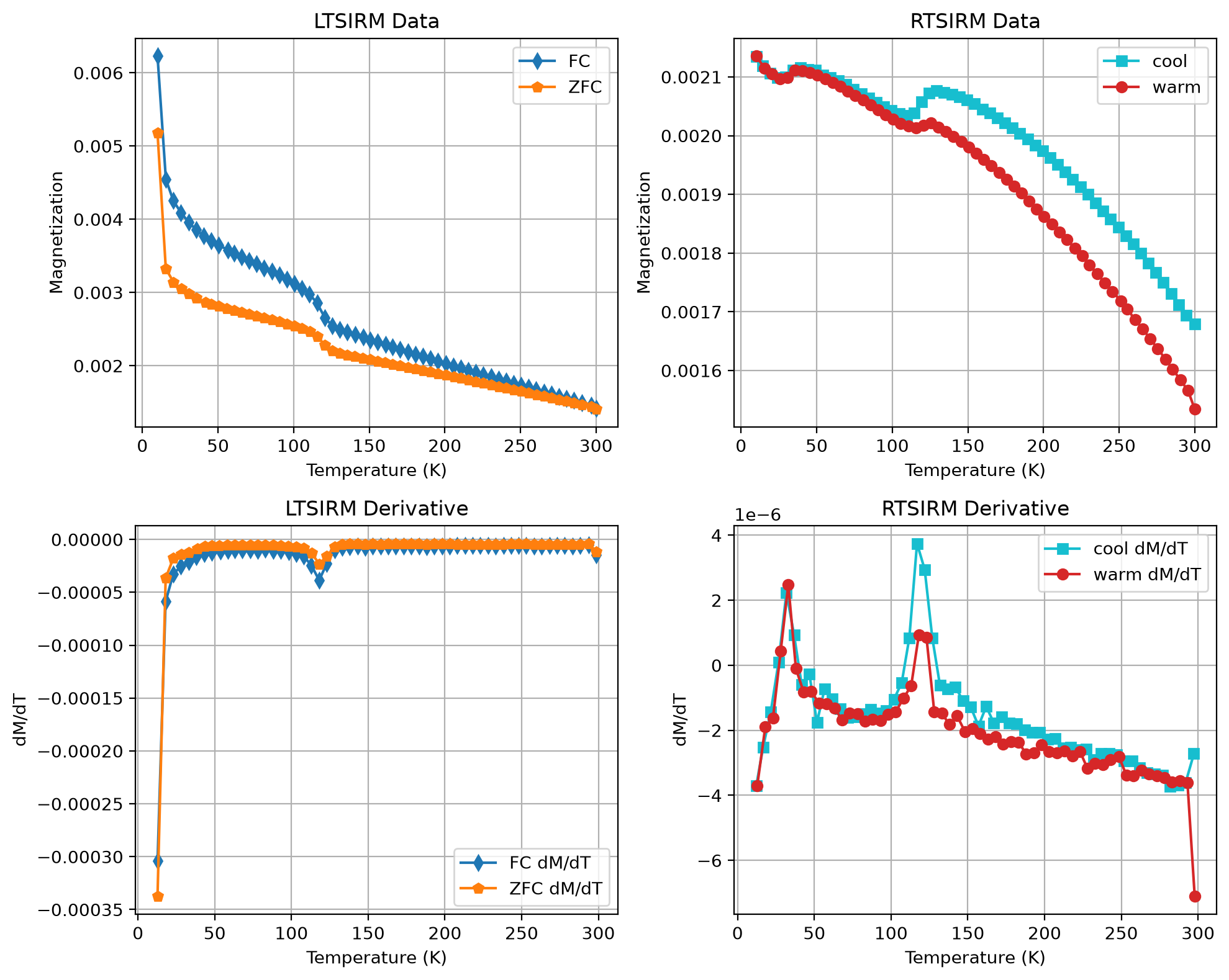
Return and save the figure
By setting return_figure=True, the figure object is returned which allows it to be saved.
figure = rmag.plot_mpms_dc(fc_data, zfc_data, rtsirm_cool_data, rtsirm_warm_data,
                           plot_derivative=True, return_figure=True)
figure.savefig('mpms_dc_plot.pdf', bbox_inches='tight')
Make interactive plots
Rather than the static plots made above (which are made using matplotlib), you may want to make interactive plots where you can zoom in and out and see the values of individual points. This can be done by putting in the parameter interactive=True which generates plots using Bokeh.
rmag.plot_mpms_dc(fc_data, zfc_data, rtsirm_cool_data, rtsirm_warm_data, interactive=True)In the plots below, the derivative is also plotted and the first and last points are dropped given issues with first point artifacts.
rmag.plot_mpms_dc(fc_data, zfc_data, rtsirm_cool_data, rtsirm_warm_data, interactive=True, plot_derivative=True, drop_first=True, drop_last=True)Symbol customization
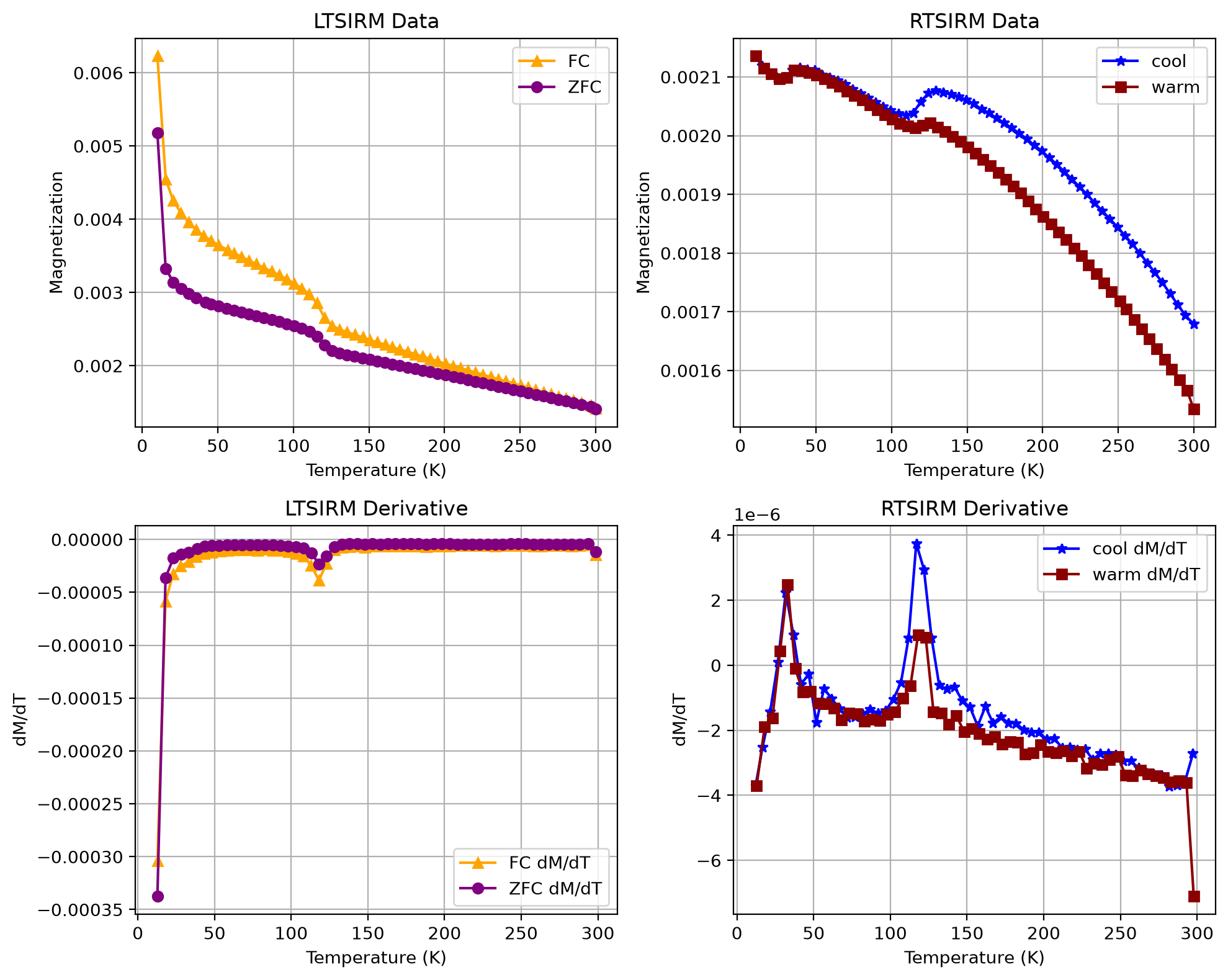
The colors and symbols of the plots can be customized by providing other values than the default parameters as in the example below:
rmag.plot_mpms_dc(fc_data, zfc_data, rtsirm_cool_data, rtsirm_warm_data,
                   fc_color='orange', zfc_color='purple', rtsirm_cool_color='blue', rtsirm_warm_color='darkred',
                   fc_marker='^', zfc_marker='o', rtsirm_cool_marker='*', rtsirm_warm_marker='s',
symbol_size=5, interactive=True)This customization can also be applied to Matplotlib plots:
rmag.plot_mpms_dc(fc_data, zfc_data, rtsirm_cool_data, rtsirm_warm_data,
                   fc_color='orange', zfc_color='purple', rtsirm_cool_color='blue', rtsirm_warm_color='darkred',
                   fc_marker='^', zfc_marker='o', rtsirm_cool_marker='*', rtsirm_warm_marker='s',
                   symbol_size=4, interactive=False, plot_derivative=True)