Hysteresis Processing walkthrough notebook

This notebook provides a step-by-step walk through of the processing of hysteresis loops. Each processing step is illustrated and described. This walk through can enable more granular data processing and illustrates the decision tree that is automatically implemented in the hysteresis_processing.ipynb.

Install and import packages¶

Import local data in MagIC format¶

In this demonstration we will be using local data.

The data is from the following publication:

• Swanson-Hysell, N. L., Avery, M. S., Zhang, Y., Hodgin, E. B., Sherwood, R. J., Apen, F. E., et al. (2021). The paleogeography of Laurentia in its early years: New constraints from the Paleoproterozoic East-Central Minnesota Batholith. Tectonics, 40, e2021TC006751. https://doi.org/10.1029/2021TC006751

Get hysteresis data from the measurements dataframe¶

The method codes relevant to hysteresis loops are:

• LP-HYS for regular hysteresis loops

• LP-HYS-O for hysteresis loops as a function of orientation

• LP-HYS-T for hysteresis loops as a function of temperature

Inspect the original measurement level data¶

• Below we investigate all the available specimens that have hysteresis data in the database for this contribution.

• We extract the experimental data for an individual specimen.

Let’s take a look at the columns relevant to hysteresis data processing

• magn_mass is mass normalized magnetization (in Am^2/kg)

• meas_field_dc is the applied DC field (in T)

Visualize the raw data with plot_hyst_loop¶

• The function returns a Bokeh plot object which can be further customized before displaying

Loop processing¶

rockmagpy calculates the hysteresis loop parameters as available in the IRMDB software. Summary parameters can then be exported into the MagIC specimen data table.

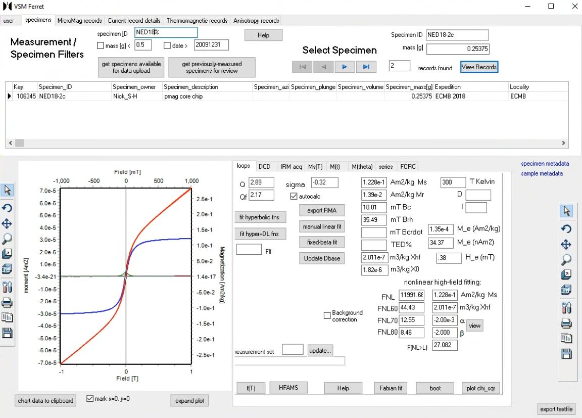
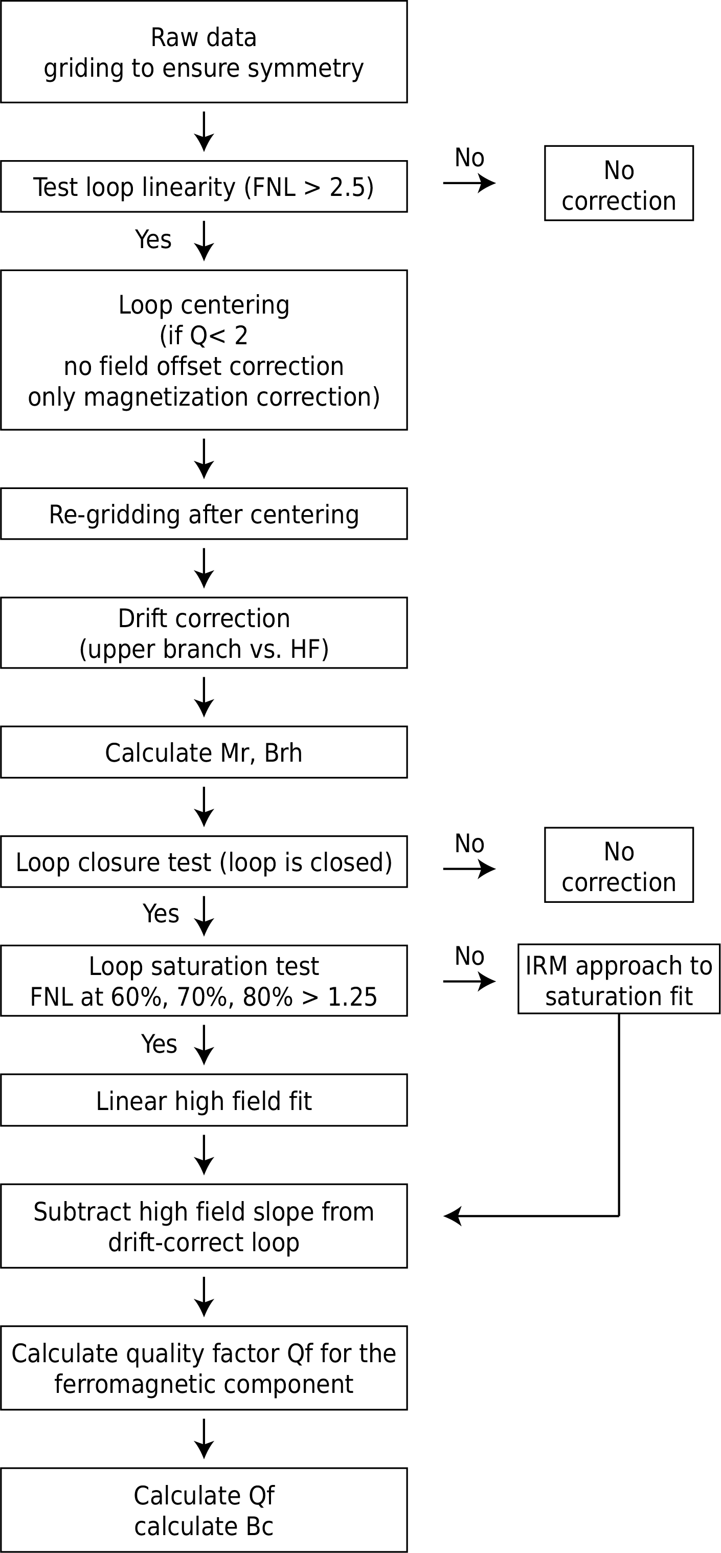
The processing functions implement the protocol of Jackson and Solheid (2010) as realized in the hysteresis processing software of the Institute for Rock Magnetism (IRM). Paterson et al. (2018) present a related treatment of hysteresis data processing (implemented in HystLab) that is a complementary resource. This flowchart shows the decision tree for data processing.

Interpolate the raw data and re-grid them into an upper and a lower branch with exactly the same and symmetric field steps¶

• The applied DC field values through the upper and lower branches during experiments are usually not exactly symmetric about the origin. We need to correct for the slight mismatching between the field steps by splitting the loop into an upper branch and a lower branch, interpolating the branches and unifying their field axis to be the same and be symmetric about 0.

• The function rmag.grid_hyst_loop accomplishes this task.

Perform linearity test on the whole loop¶

• If the whole loop is linear, the sample is dominated by paramagnetic or diamagnetic materials and no ferromagnetic parameters can be estimated (the high-field slope is the result to report).

• If the whole loop is not linear, we should move on to further processing.

• The FNL statistic is a lack-of-fit F ratio from an ANOVA partition in which the upper branch and the inverted lower branch are treated as replicate measurements (Jackson and Solheid, 2010). FNL values above ~1.25 reject whole-loop linearity at 95% confidence for typical loop sizes.

• The resulting stats dictionary from the hyst_linearity_test function has a key loop_is_linear with a boolean value that signals whether the loop is linear or not.

• process_hyst_loop implements this as a decision-tree exit: a statistically linear loop terminates with only χ_HF reported (from the whole-loop regression) and the ferromagnetic parameters as NaN. Passing fit_linear_loop=True overrides the exit and processes the loop in full, which can be useful when a weak ferromagnetic signal near the noise level is of interest.

Loop centering¶

• In the example case, the loop is not linear, so we need to isolate the ferromagnetic component from the paramagnetic component.

• We need to center the loop to remove any offset in the field and moment axes that could be present in the data.

Quality factor Q¶

Once the loop has been centered, the quality factor Q can be calculated. Following Jackson and Solheid (2010), Q is the decimal log of the signal/noise ratio, where the noise is quantified from the mean square mismatch between symmetrically equivalent moments of the offset-corrected loop. The convention used is $Q = \log_{10}(1/\sqrt{1-R^2})$, matching the IRM’s processing software and HystLab (Paterson et al., 2018, eq. 4); note that the corresponding equation as printed in Jackson and Solheid (2010) omits the square root, although the values reported in that paper include it (see Paterson et al., 2018). A higher value indicates better quality data. Note this value can deviate from that currently calculated in the IRM VSM Ferret as that value is estimated from the FNL statistic.

High Q values (e.g., 2 or greater) indicate that deviations from inversion symmetry due to all possible sources (noise, drift, and inherent asymmetry) are small. Conversely, low values indicate that at least one of these is significant. When Q falls below ~0.3 (signal/noise ~2) it becomes difficult to compute meaningful parameters for the loop, and when Q < 2 the automated processing skips the horizontal (field) offset correction because it cannot be robustly determined.

Loop drift correction¶

• Sometimes spurious changes occur in measured signal strength on time scales comparable to that of the loop measurement. Drift is typically manifested by failure of loops to close, by lack of even symmetry in M_rh, and/or by failure of M_rh to decrease to zero in large (positive or negative) fields.

• In many cases a correction is not strictly necessary as the drift signal is small. The default approach is to examine the smoothed error curve M_e (the mismatch between the upper branch and the inverted lower branch) and determine whether a high-field drift correction or an upper branch drift correction is appropriate.

• If you zoom in on the ~1 T region of the loop above, you will find that there is a slight difference between the beginning and end points.

• The Me_drift_correction function corrects the drift by subtracting a smoothed M_e curve either in the high-field region (when the largest errors occur above 75% of the maximum field) or over the entire upper branch of the loop.

Calculate the M_r (remanent magnetization), M_rh (remanence component), M_ih (induced component), M_e (error), B_rh (field corresponding to 1/2 M_r)¶

• The function calc_Mr_Mrh_Mih_Brh calculates these values and curves.

• M_rh = (M⁺ - M^-)/2 and M_ih = (M⁺ + M^-)/2 where M⁺ and M^- are the upper and lower branches; for a well-behaved loop, M_rh is an even function of field and M_ih is odd (Jackson and Solheid, 2010).

• Below we print out the M_r value and B_rh value.

Test loop closure¶

• When there are significant high coercivity components in the sample such as hematite or goethite, the hysteresis branches will not be overlapping at the highest applied fields.

• In that case, hysteresis processing stops as we are not able to estimate M_s: the ferromagnetic and linear contributions cannot be separated, so process_hyst_loop reports the slope-independent parameters (M_r and B_rh, computed from M_rh in which any linear-in-field contribution cancels) together with the data quality statistics (FNL, FNL60/70/80, Q, SNR, HAR), while M_s, χ_HF, and B_c are reported as NaN. Passing fit_open_loop=True (or NL_fit=True, which implies it) forces the high-field fit anyway---useful if residual instrument drift, rather than a genuinely open loop, trips the test.

• If the loop is closed, we move on to the next step of testing loop saturation.

• The loop_closure_test function tests loop closure using H, Mrh, and Me: the signal is the field-reflection average of M_rh in the high-field window (M_rh is an even function of field for a well-behaved loop, so this average estimates the true remanent hysteretic signal), and the noise is estimated from the high-field portion of the error curve M_e, following the implementation in HystLab (Paterson et al., 2018, section 4.5). The loop is judged closed when the high-field signal-to-noise ratio is below 8 dB or the ratio of high-field to total M_rh area is below -48 dB.

Test loop saturation (high-field linearity test)¶

• In the example case, the loop is closed, so we proceed to test the loop saturation. This test allows us to determine the appropriate approach for fitting the high-field portion of the loop and determining M_s.

• The lack of saturation can cause a loop to deviate from linearity at high fields. Although such a deviation from linearity can be subtle to the eye, it can have a significant effect on estimates of M_s. As developed in Jackson and Solheid (2010), a linearity test is conducted over high-field windows starting at 60%, 70%, and 80% of the maximum field. If the loop statistically deviates from linearity in all of these windows (FNL > 2.5), it would be inappropriate to use a linear fit to the high-field data to correct for the paramagnetic or diamagnetic slope, and an approach-to-saturation fit is required. Otherwise, a linear fit is applied over the window starting at the lowest field fraction that is statistically linear (the saturation_cutoff).

• In the example case, the loop is not saturated at 60%, 70%, and 80% of the maximum field range. Therefore, an approach to saturation fit needs to be used for isolating the ferromagnetic loop and then calculating the M_s and the high field susceptibility values.

Fit high-field slope and get the intercept as M_s¶

• In this case, the loop is not saturated at high fields and we should use an approach to saturation fit to calculate the M_s value.

• But to show the difference between a linear fit and a saturation fit, we will also perform a linear fit on the high-field data and use it to correct the loop.

• We use the linear_HF_fit function to estimate the high-field susceptibility (and the M_s intercept in the case where the loop is saturated). Note that the returned chi_HF is the fitted slope converted to SI units (multiplied by $\mu_0 = 4\pi \times 10^{-7}$).

• We then use the resultant chi_HF to correct the loop using the hyst_slope_correction function (which applies the inverse unit conversion internally).

Perform approach-to-saturation fit and estimate a more appropriate M_s¶

• In this example case, a linear fit would underestimate the M_s value.

• A more appropriate M_s value can be estimated using a nonlinear approach-to-saturation fit with the hyst_HF_nonlinear_optimization function.

• By default (fit_type='IRM'), the model used at the IRM is fit:

  $$M = \chi_{HF} H + M_s + a_1 H^{-1} + a_2 H^{-2}$$

  (1)

  Alternative model forms of $M = \chi_{HF} H + M_s + \alpha H^{\beta}$ (Fabian, 2006) are available with fit_type='Fabian' (free $\beta$) and fit_type='Fabian_fixed_beta' ($\beta = -2$).

• The returned Fnl_lin statistic (Jackson and Solheid, 2010, eq. 21) tests whether the nonlinear fit significantly improves on a linear fit; values above ~3-3.5 indicate a significant improvement.

Now let’s use the approach-to-saturation fit result to correct the loop.

Plot the ferromagnetic component together with the previous intermediate products¶

• You may click on the legend items to hide the curves

• The preferred final ferromagnetic component is shown in pink

Inspect the differences between applying a linear high field slope fit vs. an approach-to-saturation fit¶

Calculate the quality factor of the ferromagnetic component loop¶

Qf is the quality factor Q recomputed on the slope-corrected (ferromagnetic component) loop (the $Q_f$ of Jackson and Solheid, 2010). The high-field slope correction affects the mean square signal strength but not the noise, so Qf quantifies the signal/noise of the isolated ferromagnetic loop.

Calculate B_c¶

• This calculation is based on the ferromagnetic component loop.

• There will be a difference if you use the loops before high-field slope correction.

• The B_c value is calculated as the average of the lower and upper branch.

• The value shown is in unit of Tesla.

The process_hyst_loop function¶

The process_hyst_loop function applies all of the above steps using the decision tree to process the data. The summary table includes the parameters developed above as well as the hysteresis shape parameter $\sigma_{hys} = \ln[E_{hys}/(4 B_c M_s)]$ of Fabian (2003), where $E_{hys}$ is the area of the ferromagnetic loop. Options include NL_fit=True to force an approach-to-saturation fit, centering_protocol='iterative' for weak ferromagnetic loops superimposed on a strong linear background, and the decision-tree overrides fit_open_loop=True (proceed with the high-field fitting for a loop the closure test flags as open; implied by NL_fit=True) and fit_linear_loop=True (fully process a loop that passes the whole-loop linearity test).

References¶

Fabian, K. (2003). Some additional parameters to estimate domain state from isothermal magnetization measurements. Earth and Planetary Science Letters, 213(3-4), 337–345. https://doi.org/10.1016/S0012-821X(03)00329-7

Fabian, K. (2006). Approach to saturation analysis of hysteresis measurements in rock magnetism and evidence for stress dominated magnetic anisotropy in young mid-ocean ridge basalt. Physics of the Earth and Planetary Interiors, 154, 299–307. Fabian (2006)

Jackson, M., & Solheid, P. (2010). On the quantitative analysis and evaluation of magnetic hysteresis data. Geochemistry, Geophysics, Geosystems, 11(4), Q04Z15. Jackson & Solheid (2010)

Paterson, G. A., Zhao, X., Jackson, M., & Heslop, D. (2018). Measuring, processing, and analyzing hysteresis data. Geochemistry, Geophysics, Geosystems, 19(7), 1925–1945. Paterson et al. (2018)

Swanson-Hysell, N. L., Avery, M. S., Zhang, Y., Hodgin, E. B., Sherwood, R. J., Apen, F. E., et al. (2021). The paleogeography of Laurentia in its early years: New constraints from the Paleoproterozoic East-Central Minnesota Batholith. Tectonics, 40, e2021TC006751. Swanson‐Hysell et al. (2021)