Magnetic susceptibility describes the relationship between an applied magnetic field and the magnetization that is induced by this field:
where is the magnetization (in Am2/kg), is the applied field (in A/m), and is the magnetic susceptibility (this is the mass susceptibility in m3/kg). Magnetic susceptibility reflects the diamagnetic, paramagnetic, and/or ferromagnetic response of minerals within a sample.
If a material is perfectly isotropic with the magnetization response being uniform in all directions, the relationship described by is independent of the orientation of the sample relative to the applied field. In this case, is a scalar quantity (a single number). However, if there is a different response in different orientations the material can be considered to be anisotropic. In this case, needs to be described as a tensor ().
In practice, anisotropy of magnetic susceptibility (AMS) is quantified by varying the orientation of a sample within the coils of a magnetic susceptibility bridge. By doing so, the length and orientation of the principal, major, and minor eigenvectors which are defined as:
these eigenvectors are also referred to in the literature as:
and the AMS ellipsoid can be illustrated as:
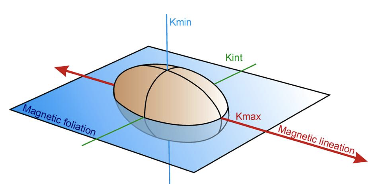
From https://www.agico.cz/downloads/documents/agicoprints/ams_rocks_pres.pdf
In the above plot, the axes of the ellipsoid are the eigenvectors (commonly referred to as the “principal axes”) with their magnitudes corresponding to the eigenvalues. Collectively, the eigenvalues and eigenvectors are called the eigenparameters. The orientation of this ellipsoid and the relative magnitude of the eigenvectors is central to the interpretation of AMS data.
The MagIC convention for the magnetic susceptibility tensor
The aniso_s list is a six-element colon-delimited list provided in the aniso_s column of a MagIC specimens tables that is a succinct representation of the anisotropy tensor . In the linear equations below, , , and are the components of the magnetization vector . The relationship between the magnetization and the magnetic field (, , and ) is described by the components of the magnetic susceptibility tensor . If the material is anisotropic, there will be different values in different orientations described by the tensor.
This susceptibility tensor has six independent matrix elements because . The aniso_s column contains these six elements as : : : : : which are defined as:
Anisotropy measurements in practice
In many laboratories, magnetic susceptibility is measured by placing a sample in a solenoid with an applied field H. The induced magnetization M parallel to H is measured in different orientations. Only s1, s2, and s3 can be measured directly. The other terms s4, s5, and s6 are only indirectly determined. For multi-positional approaches, the sets of values of measurements such as susceptibility would be where A is the design matrix.
The Jelínek 15 position diagram
Statistical processing of anisotropy of magnetic susceptibility measured on groups of specimens by Jelínek (1978) illustrates the 15 position scheme of anisotropy measurement.
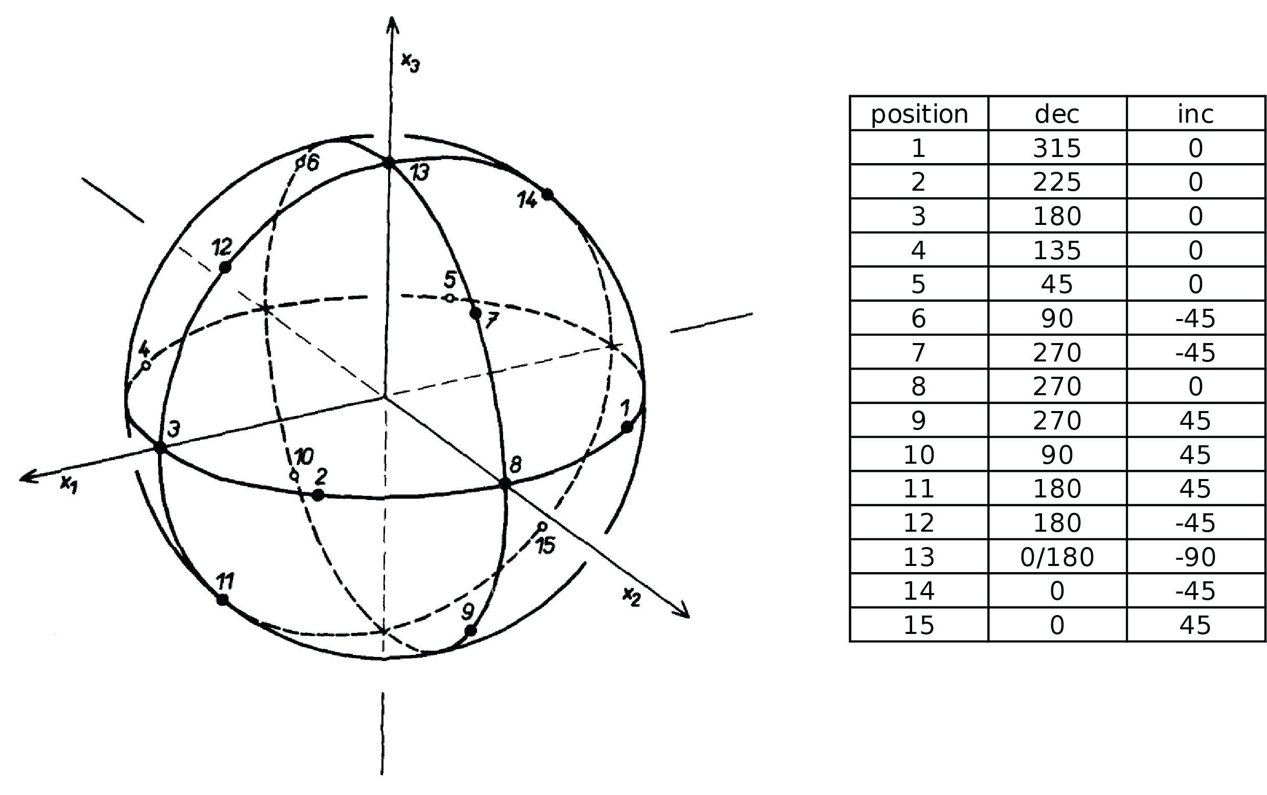
It is also possible to adopt a 9-position experimental approach. In this case, follow positions 1,2,3, 6,7,8, 11,12,13 of the Jelínek 15 position scheme for the anisotropy experiments.
The 15-position design matrix is given by:
This 15-position procedure is widely adopted in experiments that seek to quantify the AMS tensor.